Iliad Intensive Curriculum

What you’ll learn

Formalize the agent-environment interaction, value functions, and the Bayes-optimal policy that defines AIXI.
Derive the explicit expectimax form of AIXI.
Prove on-policy value convergence and that AIXI cannot be fooled in deterministic environments.
Prove the self-optimizing property via likelihood-ratio martingales and change of measure.

Much of this material is drawn from (Hutter et al. 2024). The book provides fuller explanations, additional context, and proofs omitted here.

Difficulty ratings. Each subproblem is tagged with a rating in square brackets using Knuth's scale (Knuth 1973): roughly, [00] trivial, [10] 15–minute pencil-and-paper, [20] 1–2 hours, [30] several hours to a day, [40] a significant research result. Intermediate values are possible. See Appendix B for the full scale.

Problems marked ( $*$ ) are less interesting/insightful and while the result may be used later, I would recommend skipping them on a first pass.

Overview

AIXI is the action half of Universal AI: it lifts the Bayesian mixture from Solomonoff induction — learning to predict — to learning to act. Now the agent takes actions that shape what it observes, and AIXI is the Bayes-optimal policy over a universal mixture $ξ$ of environments. It learns to act as well as if it knew the true environment $μ$ . Under the universal choice — $M$ = all lower-semicomputable environments, prior $w_{ν} = 2^{- K (ν)}$ — the assumption " $μ \in M$ " again becomes "the universe is computable."

Prerequisites

Solomonoff Induction — start there first. The Bayesian mixture, posterior updates, and dominance carry over directly; AIXI reuses them in the action setting.
Comfort with discrete probability (conditional distributions, chain rule, expectations).
Familiarity with sequential decision-making / reinforcement learning (agents, rewards, discounting, value functions) is useful but not assumed.

Goal and Roadmap

This exercise sheet builds towards three main results:

On-policy value convergence (Section 7): the Bayesian mixture $ξ$ learns to predict the value of any fixed policy as well as the true environment $μ$ .
AIXI can't be fooled (Section 8): in deterministic environments, the Bayes-optimal agent is guaranteed non-zero value whenever optimal value is non-zero.
Self-optimizing property (Section 11, advanced stretch goal): the Bayes-optimal policy $π_{ξ}^{*}$ learns to act as well as if it knew $μ$ , provided that any learnable policy can achieve this. This is the central theoretical justification for the AIXI agent.

A good target is to complete Section 7 and 8. The self-optimizing property (Sections 9–11) requires substantial additional machinery (supermartingales, change of measure) and is an advanced stretch goal.

Critical path. The three results share a common foundation (Sections 0–4) and then diverge:

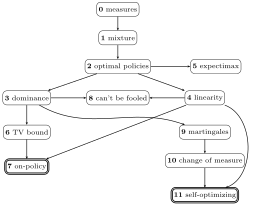
In summary:

Sections 0–4 establish the Bayesian RL framework: measure algebra, mixture properties, existence of optimal policies, dominance, and linearity.
Section 5 derives the explicit expectimax form of AIXI.
Sections 6–7 prove on-policy value convergence: $V_{ξ}^{π}$ and $V_{μ}^{π}$ become indistinguishable for any fixed $π$ .
Section 8 shows AIXI can't be fooled: the Bayes-optimal agent achieves non-zero value whenever optimal value is non-zero (in deterministic environments).
Sections 9–11 (advanced stretch goal) prove the self-optimizing property: if any policy can learn to act optimally, $π_{ξ}^{*}$ inherits this.

Setup

An agent interacts with an environment in discrete time steps $t = 1, 2, \dots$ .

Definition 0.1 (Spaces and notation). - $A$ : finite set of actions

$O$ : finite set of observations
$R \subset [0, 1]$ : finite set of rewards
$E := O \times R$ : set of percepts; $e_{t} = (o_{t}, r_{t}) \equiv o_{t} r_{t}$
$H^{t} := (A \times E)^{t}$ : set of all histories of length $t$
$H^{*} := \cup_{t = 0}^{\infty} H^{t}$ : set of all finite histories
$H^{\infty} := (A \times E)^{\infty}$ : set of all infinite histories
$Δ S$ : set of all probability distributions over set $S$
$[[\cdot]]$ : Iverson bracket: $[[P]] = 1$ if $P$ is true, $0$ if false
$t$ : current time step; $m$ : finite horizon; $1 \leq t \leq m$
$i, j, k$ : arbitrary integer indices
$x y$ : concatenation
$ϵ$ : the empty string/history
$æ_{i : j} := a_{i} e_{i} a_{i + 1} e_{i + 1} \dots a_{j} e_{j}$ : history segment from time $i$ to $j$
$æ_{< t} := a_{1} e_{1} a_{2} e_{2} \dots a_{t - 1} e_{t - 1}$ : history up to (but not including) time $t$

Definition 0.2 (Policy $π$ ). A policy $π : H \to Δ A$ maps each history to a probability distribution over actions. Given history $æ_{< t}$ :

$π (\cdot ∣ æ_{< t})$ is a distribution over $A$ ,
$π (a_{t} ∣ æ_{< t}) \in [0, 1]$ is the probability of choosing action $a_{t}$ ,
the agent samples $a_{t} \sim π (\cdot ∣ æ_{< t})$ .

A policy is deterministic if $π (a ∣ æ_{< t}) \in {0, 1}$ for all $a, æ_{< t}$ . We write $π (æ_{i : j}) := \prod_{k = i}^{j} π (a_{k} ∣ æ_{< k})$ .

Definition 0.3 (Environment $ν$ ). An environment $ν : H \times A \to Δ E$ maps each history–action pair to a distribution over percepts. Given history $æ_{< t}$ and action $a_{t}$ :

$ν (\cdot ∣ æ_{< t} a_{t})$ is a distribution over $E$ ,
$ν (e_{t} ∣ æ_{< t} a_{t}) \in [0, 1]$ is the probability of percept $e_{t}$ ,
the environment samples $e_{t} \sim ν (\cdot ∣ æ_{< t} a_{t})$ .

We write $ν (æ_{i : j}) := \prod_{k = i}^{j} ν (e_{k} ∣ æ_{< k} a_{k})$ . This satisfies the chain rule: $ν (æ_{i : j}) = ν (æ_{i : j - 1}) \cdot ν (e_{j} ∣ æ_{i : j - 1} a_{j})$ or in the form we will usually use, $ν (æ_{1 : t}) = ν (æ_{< t}) \cdot ν (e_{t} ∣ æ_{< t} a_{t})$ . An environment is deterministic if $ν (e_{t} ∣ æ_{< t} a_{t}) \in {0, 1}$ for all $e_{t}, æ_{< t}, a_{t}$ (each percept is produced with certainty). We denote the true (unknown) environment by $μ$ .

Definition 0.4 (Interaction measure $ν^{π}$ ). When policy $π$ interacts with environment $ν$ , the joint probability of a history segment $æ_{i : j}$ given past $æ_{< i}$ is

ν^{π} (æ_{i : j} ∣ æ_{< i}) := k = i \prod j π (a_{k} ∣ æ_{< k}) ν (e_{k} ∣ æ_{< k} a_{k}) .

0. Properties of Measures

Exercise 0.1 (Factorization) [05]. Show that $ν^{π} (æ_{1 : t}) = π (æ_{1 : t}) \cdot ν (æ_{1 : t})$ .

Solution

Expanding the definition: $ν^{π} (æ_{1 : t}) = \prod_{k = 1}^{t} π (a_{k} ∣ æ_{< k}) ν (e_{k} ∣ æ_{< k} a_{k}) = π (æ_{1 : t}) k = 1 \prod t π (a_{k} ∣ æ_{< k}) \cdot ν (æ_{1 : t}) k = 1 \prod t ν (e_{k} ∣ æ_{< k} a_{k})$ .

Key observation: $π (æ_{1 : t})$ is the same regardless of the environment. When comparing $ν^{π}$ and $μ^{π}$ , the policy factors cancel.

Exercise 0.2 (Chain rule) [05]. Show that $ν (æ_{1 : t}) = ν (æ_{< t}) \cdot ν (e_{t} ∣ æ_{< t} a_{t})$ .

Solution

From the definition $ν (æ_{1 : t}) = \prod_{k = 1}^{t} ν (e_{k} ∣ æ_{< k} a_{k})$ , split off the last factor:

ν (æ_{1 : t}) = k = 1 \prod t - 1 ν (e_{k} ∣ æ_{< k} a_{k}) \cdot ν (e_{t} ∣ æ_{< t} a_{t}) = ν (æ_{< t}) \cdot ν (e_{t} ∣ æ_{< t} a_{t}) .

Exercise 0.3 (∗) (Marginalizing percepts) [03]. Show that $\sum_{e_{t}} ν^{π} (a_{t} e_{t} ∣ æ_{< t}) = π (a_{t} ∣ æ_{< t})$ .

Solution

From Definition 0.4, the one-step interaction is $ν^{π} (a_{t} e_{t} ∣ æ_{< t}) = π (a_{t} ∣ æ_{< t}) ν (e_{t} ∣ æ_{< t} a_{t})$ . Summing over $e_{t}$ :

e_{t} \sum ν^{π} (a_{t} e_{t} ∣ æ_{< t}) = π (a_{t} ∣ æ_{< t}) = 1 e_{t} \sum ν (e_{t} ∣ æ_{< t} a_{t}) = π (a_{t} ∣ æ_{< t}) .

Interpretation: after summing out the environment's response, only the agent's action probability remains.

Exercise 0.4 (∗) (Deterministic interaction measure) [05]. Let $π$ be a deterministic policy, i.e. at each history $æ_{< k}$ there is a unique action $a_{k}^{*}$ with $π (a_{k}^{*} ∣ æ_{< k}) = 1$ . Show that, provided $æ_{i : j}$ is consistent with $π$ (i.e. $a_{k} = a_{k}^{*}$ for every $k \in {i, \dots, j}$ ):

ν^{π} (æ_{i : j} ∣ æ_{< i}) = ν (æ_{i : j} ∣ æ_{< i}),

i.e. on $π$ -consistent futures the interaction measure reduces to the environment measure: every policy factor is $1$ .

Solution

Since $π$ is deterministic, $π (a_{k} ∣ æ_{< k}) = [[a_{k} = a_{k}^{*}]]$ . By hypothesis $æ_{i : j}$ is $π$ -consistent, so every such bracket equals $1$ . From Definition 0.4:

ν^{π} (æ_{i : j} ∣ æ_{< i}) = k = i \prod j = 1 π (a_{k} ∣ æ_{< k}) ν (e_{k} ∣ æ_{< k} a_{k}) = k = i \prod j ν (e_{k} ∣ æ_{< k} a_{k}) = ν (æ_{i : j} ∣ æ_{< i}),

where the last equality is the natural segment extension of $ν (æ_{1 : t}) := \prod_{k = 1}^{t} ν (e_{k} ∣ æ_{< k} a_{k})$ .

Exercise 0.5 [05]. (General chain rule for $ν^{π}$ ) Show that for any $p \leq q \leq r$ :

ν^{π} (æ_{p : r} ∣ æ_{< p}) = ν^{π} (æ_{p : q} ∣ æ_{< p}) \cdot ν^{π} (æ_{q + 1 : r} ∣ æ_{< p} æ_{p : q}) .

Solution

Split the defining product $ν^{π} (æ_{p : r} ∣ æ_{< p}) = \prod_{k = p}^{r} π (a_{k} ∣ æ_{< k}) ν (e_{k} ∣ æ_{< k} a_{k})$ at index $q$ :

ν^{π} (æ_{p : r} ∣ æ_{< p}) = k = p \prod r π (a_{k} ∣ æ_{< k}) ν (e_{k} ∣ æ_{< k} a_{k}) = ν^{π} (æ_{p : q} ∣ æ_{< p}) k = p \prod q π (a_{k} ∣ æ_{< k}) ν (e_{k} ∣ æ_{< k} a_{k}) \cdot ν^{π} (æ_{q + 1 : r} ∣ æ_{< p} æ_{p : q}) k = q + 1 \prod r π (a_{k} ∣ æ_{< k}) ν (e_{k} ∣ æ_{< k} a_{k}),

identifying each block as a conditional via the same expansion: the past for step $k \geq q + 1$ is the given history $æ_{< p}$ extended by the first chunk $æ_{p : q}$ .

Note: for a deterministic policy, Exercise 0.4 simplifies this further: each factor $π (a_{k} ∣ æ_{< k}) ν (e_{k} ∣ æ_{< k} a_{k})$ becomes just $ν (e_{k} ∣ æ_{< k} a_{k}^{*})$ .

The Bayesian Mixture and Value Function

Definition 0.1 (Model class, prior, and Bayesian mixture $ξ$ ). Let $M = {ν_{1}, ν_{2}, \dots}$ be a countable class of environments with prior weights $w_{ν} > 0$ satisfying $\sum_{ν \in M} w_{ν} \leq 1$ . We assume $μ \in M$ .

The Bayesian mixture $ξ$ is defined as

ξ (æ_{1 : t}) := ν \in M \sum w_{ν} ν (æ_{1 : t}) and ξ (e_{t} ∣ æ_{< t} a_{t}) := ξ (æ_{1 : t}) / ξ (æ_{< t}) .

One can show that the one-step predictive distribution can be written as

ξ (e_{t} ∣ æ_{< t} a_{t}) = ν \in M \sum w (ν ∣ æ_{< t}) ν (e_{t} ∣ æ_{< t} a_{t}),

where the posterior weight is

w (ν ∣ æ_{< t}) := w_{ν} \frac{ν ( æ _{< t} )}{ξ ( æ _{< t} )}, w (ν ∣ ϵ) := w_{ν} .

See Appendix A for a worked example.

Definition 0.2 (Expectation $E_{ν}^{π}$ ). For a function $f : H \to R$ of a finite future segment $æ_{t : m}^{'}$ :

E_{ν}^{π} [f ∣ æ_{< t}] := æ_{t : m} \sim ν^{π} (\cdot ∣ æ_{< t}) E [f] = æ_{t : m}^{'} \sum ν^{π} (æ_{t : m}^{'} ∣ æ_{< t}) f (æ_{t : m}^{'}) .

For functions $f$ of the infinite future (like the value function), with a sequence $f_{1}, f_{2}, \dots \to f$ , where $f_{m}$ depends only on $æ_{t : m}^{'}$ , we define $E_{ν}^{π} [f ∣ æ_{< t}] := lim_{m \to \infty} E_{ν}^{π} [f_{m} ∣ æ_{< t}]$ ,

Definition 0.3 (Discounted return $G_{t : m}$ ). Fix a discount factor $γ \in (0, 1)$ , held constant throughout. The discounted return at time step $t$ , up to horizon $m$ , is

G_{t : m}^{γ} := k = t + 1 \sum m γ^{k - (t + 1)} r_{k} = r_{t + 1} + γ r_{t + 2} + \dots + γ^{m - t} r_{m} .

Since $γ$ is fixed we drop it and write $G_{t : m} \equiv G_{t : m}^{γ}$ . It satisfies the recursion $G_{t : m} = r_{t + 1} + γ G_{t + 1 : m}$ , with $G_{m - 1 : m} = r_{m}$ and $G_{n : m} = 0$ for $n \geq m$ . The infinite-horizon return is the pointwise limit

G_{\geq t} \equiv G_{t : \infty} := m \to \infty lim G_{t : m} = k = t + 1 \sum \infty γ^{k - (t + 1)} r_{k},

with the clean recursion $G_{\geq t} = r_{t + 1} + γ G_{\geq t + 1}$ and no boundary cases.

Definition 0.4 (Value function¹). The value of policy $π$ in environment $ν$ with horizon $m \geq t$ given history $æ_{< t}$ is

V_{ν}^{π, m} (æ_{< t}) := (1 - γ) E_{ν}^{π} [G_{t - 1 : m} ∣ æ_{< t}] = (1 - γ) æ_{t : m} \sum ν^{π} (æ_{t : m} ∣ æ_{< t}) G_{t - 1 : m} = (1 - γ) æ_{t : m} \sum ν^{π} (æ_{t : m} ∣ æ_{< t}) [k = t \sum m γ^{k - t} r_{k}] .

The infinite-horizon value is the pointwise limit $V_{ν}^{π, \infty} (æ_{< t}) := lim_{m \to \infty} V_{ν}^{π, m} (æ_{< t}) = (1 - γ) E_{ν}^{π} [G_{\geq t - 1} ∣ æ_{< t}]$ . We write $V_{ν}^{π} \equiv V_{ν}^{π, \infty}$ for short.

The optimal value is $V_{ν}^{*, m} (æ_{< t}) := sup_{π} V_{ν}^{π, m} (æ_{< t})$ for $m \in N \cup {\infty}$ , with $V_{ν}^{*} \equiv V_{ν}^{*, \infty}$ . ² An optimal policy $π_{ν}^{*}$ satisfies $V_{ν}^{π_{ν}^{*}} = V_{ν}^{*}$ . The Bayes-optimal policy is $π_{ξ}^{*} \in arg max_{π} V_{ξ}^{π}$ .

Remark (AIXI). All results in this sheet hold for any countable $M$ and prior weights $w_{ν}$ . AIXI is a special case of the Bayes-optimal policy $π_{ξ}^{*}$ for the particular choice $M :=$ the class of all lower-semicomputable chronological semimeasures, and prior $w_{ν} := 2^{- K (ν)}$ , where $K (ν)$ is the Kolmogorov complexity of $ν$ : the length of the shortest program that computes $ν$ . The resulting agent is written $π_{ξ_{U}}^{*}$ , or simply AI $ξ$ .

Why this $M$ ? By including every computable environment, the assumption $μ \in M$ reduces to "the universe is computable": as weak an assumption as one can make.

Why this prior? The prior $2^{- K (ν)}$ is dominant: for any other computable prior $w_{ν}^{'}$ , there exists a constant $c > 0$ such that $2^{- K (ν)} \geq c \cdot w_{ν}^{'}$ for all $ν$ .

Caveat: The constant $c$ depends on the choice of universal Turing machine $U$ , and adversarial choices of $U$ can make AIXI behave arbitrarily badly (Leike & Hutter 2015).

See (Hutter et al. 2024): Chapter 2.7 for Kolmogorov complexity, Chapters 3.7–3.8 for the model class and universal prior, and Chapter 7.4 for AIXI itself.

1. Properties of the Bayesian Mixture

Exercise 1.1 (∗) (Posterior update) [10]. Show that the posterior updates multiplicatively:

w (ν ∣ æ_{1 : t}) = w (ν ∣ æ_{< t}) \frac{ν ( e _{t} ∣ æ _{< t} a _{t} )}{ξ ( e _{t} ∣ æ _{< t} a _{t} )} .

Hint

Use the definitions of $w (ν ∣ æ_{1 : t})$ and $w (ν ∣ æ_{< t})$ , and apply Exercise 0.2.

Solution

From the definition: $w (ν ∣ æ_{1 : t}) = w_{ν} \cdot ν (æ_{1 : t}) / ξ (æ_{1 : t})$ and $w (ν ∣ æ_{< t}) = w_{ν} \cdot ν (æ_{< t}) / ξ (æ_{< t})$ .

Dividing:

\frac{w ( ν ∣ æ _{1 : t} )}{w ( ν ∣ æ _{< t} )} = \frac{ν ( æ _{1 : t} )}{ν ( æ _{< t} )} \cdot \frac{ξ ( æ _{< t} )}{ξ ( æ _{1 : t} )} = \frac{ν ( e _{t} ∣ æ _{< t} a _{t} )}{ξ ( e _{t} ∣ æ _{< t} a _{t} )},

where we used the chain rule (Exercise 0.2) for both $ν$ and $ξ$ .

Exercise 1.2 [15]. (One-step predictive distribution of $ξ$ ) Starting from $ξ (æ_{1 : t}) = \sum_{ν \in M} w_{ν} ν (æ_{1 : t})$ , derive the one-step predictive form:

ξ (e_{t} ∣ æ_{< t} a_{t}) = ν \in M \sum w (ν ∣ æ_{< t}) ν (e_{t} ∣ æ_{< t} a_{t}) .

Hint

Write $ξ (e_{t} ∣ æ_{< t} a_{t}) = ξ (æ_{1 : t}) / ξ (æ_{< t})$ , expand the numerator, and use Exercise 0.2.

Solution

The one-step conditional is the ratio of joint to marginal: $ξ (e_{t} ∣ æ_{< t} a_{t}) := ξ (æ_{1 : t}) / ξ (æ_{< t})$ .

Expanding the numerator using $ξ (æ_{1 : t}) = \sum_{ν} w_{ν} ν (æ_{1 : t})$ :

ξ (e_{t} ∣ æ_{< t} a_{t}) = \frac{\sum _{ν \in M} w _{ν} ν ( æ _{1 : t} )}{ξ ( æ _{< t} )} = \frac{\sum _{ν} w _{ν} ν ( æ _{< t} ) \cdot ν ( e _{t} ∣ æ _{< t} a _{t} )}{ξ ( æ _{< t} )} (chain rule, Exercise 0.2) = ν \sum = w (ν ∣ æ_{< t}) \frac{w _{ν} ν ( æ _{< t} )}{ξ ( æ _{< t} )} \cdot ν (e_{t} ∣ æ_{< t} a_{t}) = ν \in M \sum w (ν ∣ æ_{< t}) ν (e_{t} ∣ æ_{< t} a_{t}) .

Exercise 1.3 (Bounded value) [10]. Show that $V_{ν}^{π, m} (æ_{< t}) \in [0, 1]$ for any $ν, π, m \in N \cup {\infty}, æ_{< t}$ .

Hint

Recall the formula for geometric series: $(1 - γ) \sum_{k = 0}^{n} γ^{k} = 1 - γ^{n + 1}$ .

Solution

Since $r_{k} \in [0, 1]$ , each discounted reward sum is bounded:

0 \leq (1 - γ) G_{t - 1 : m} \leq (1 - γ) k = t \sum m γ^{k - t} = 1 - γ^{m - t + 1} \leq 1.

The interaction measure satisfies $ν^{π} (æ_{t : m}^{'} ∣ æ_{< t}) \geq 0$ and $\sum_{æ_{t : m}^{'}} ν^{π} (æ_{t : m}^{'} ∣ æ_{< t}) = 1$ , so the value function is a weighted average of terms in $[0, 1]$ :

0 \leq V_{ν}^{π, m} (æ_{< t}) = æ_{t : m}^{'} \sum ν^{π} (æ_{t : m}^{'} ∣ æ_{< t}) (1 - γ) G_{t - 1 : m} \leq 1.

For $m = \infty$ : since $0 \leq V_{ν}^{π, m} (æ_{< t}) \leq 1$ for all finite $m$ , the limit $V_{ν}^{π} (æ_{< t}) = lim_{m \to \infty} V_{ν}^{π, m} (æ_{< t})$ also lies in $[0, 1]$ .

Exercise 1.4 (∗) [15]. (Multi-step posterior linearity of $ξ^{π}$ ) Extend Exercise 1.2 to multi-step histories: show that for finite $m \geq t$ ,

ξ^{π} (æ_{t : m} ∣ æ_{< t}) = ν \in M \sum w (ν ∣ æ_{< t}) ν^{π} (æ_{t : m} ∣ æ_{< t}) .

Hint

Apply the general chain rule (Exercise 0.5) to $ξ (æ_{1 : m}) = \sum_{ν} w_{ν} ν (æ_{1 : m})$ , then use factorization (Exercise 0.1).

Solution

Start from the definition $ξ (æ_{1 : m}) = \sum_{ν \in M} w_{ν} ν (æ_{1 : m})$ . Apply the general chain rule (Exercise 0.5) to both sides: $ξ (æ_{1 : m}) = ξ (æ_{< t}) \cdot ξ (æ_{t : m} ∣ æ_{< t})$ and $ν (æ_{1 : m}) = ν (æ_{< t}) \cdot ν (æ_{t : m} ∣ æ_{< t})$ . Dividing by $ξ (æ_{< t})$ :

ξ (æ_{t : m} ∣ æ_{< t}) = ν \in M \sum \frac{w _{ν} ν ( æ _{< t} )}{ξ ( æ _{< t} )} ν (æ_{t : m} ∣ æ_{< t}) = ν \in M \sum w (ν ∣ æ_{< t}) ν (æ_{t : m} ∣ æ_{< t}) .

Now multiply both sides by $π (æ_{t : m} ∣ æ_{< t})$ . By factorization (Exercise 0.1), $π (æ_{t : m} ∣ æ_{< t}) \cdot ξ (æ_{t : m} ∣ æ_{< t}) = ξ^{π} (æ_{t : m} ∣ æ_{< t})$ and likewise for each $ν$ :

ξ^{π} (æ_{t : m} ∣ æ_{< t}) = ν \in M \sum w (ν ∣ æ_{< t}) ν^{π} (æ_{t : m} ∣ æ_{< t}) .

2. Existence of Optimal Policies

Recall that $V_{ν}^{*} (æ_{< t}) := sup_{π} V_{ν}^{π} (æ_{< t})$ is defined as a supremum over all policies. In general, a supremum need not be achieved: for example, $sup_{x \in (0, 1)} x = 1$ , but no $x \in (0, 1)$ attains this value. This problem shows that in our setting, the supremum is attained, so an optimal policy $π_{ν}^{*}$ with $V_{ν}^{π_{ν}^{*}} = V_{ν}^{*}$ exists.

Exercise 2.1 [05]. Consider a single time step. Given history $æ_{< t}$ and a function $Q : A \to R$ , show that $sup_{π} \sum_{a \in A} π (a ∣ æ_{< t}) Q (a) = max_{a \in A} Q (a)$ , and that the supremum is attained by the deterministic policy that places all probability on an action achieving the maximum.

Solution

Let $a^{*} \in arg max_{a^{'} \in A} Q (a^{'})$ , which exists because $A$ is finite. So $Q (a^{*}) = max_{a^{'}} Q (a^{'})$ .

Upper bound. For any $π$ : $\sum_{a} π (a ∣ æ_{< t}) Q (a) \leq \sum_{a} π (a ∣ æ_{< t}) Q (a^{*}) = Q (a^{*})$ .

Lower bound. The deterministic $π^{*}$ with $π^{*} (a^{*} ∣ æ_{< t}) = 1$ achieves $Q (a^{*})$ .

Combining: $sup_{π} \sum_{a} π (a) Q (a) = Q (a^{*}) = max_{a^{'}} Q (a^{'})$ , attained by $π^{*}$ .

Exercise 2.2 (Bellman equation) [15]. Show that for finite $m$ and $t \leq m$ :

V_{ν}^{π, m} (æ_{< t}) = æ_{t}^{'} \sum ν^{π} (æ_{t}^{'} ∣ æ_{< t}) [(1 - γ) r_{t}^{'} + γ V_{ν}^{π, m} (æ_{< t} æ_{t}^{'})],

Hint

Use the general chain rule (Exercise 0.5) to peel off the first step,

ν^{π} (æ_{t : m} ∣ æ_{< t}) = ν^{π} (æ_{t} ∣ æ_{< t}) \cdot ν^{π} (æ_{t + 1 : m} ∣ æ_{1 : t}) .

Break up the sum $\sum_{æ_{t : m}} = \sum_{æ_{t}} \sum_{æ_{t + 1 : m}}$ , and factor out $r_{t}^{'}$ using $\sum_{æ_{t + 1 : m}^{'}} ν^{π} (æ_{t + 1 : m}^{'} ∣ æ) = 1$ for any history $æ$ .

Solution

Step 1: Factor the future. Write $æ_{t : m}^{'} = æ_{t}^{'} æ_{t + 1 : m}^{'}$ : $ν^{π} (æ_{t : m}^{'} ∣ æ_{< t}) = ν^{π} (æ_{t}^{'} ∣ æ_{< t}) \cdot ν^{π} (æ_{t + 1 : m}^{'} ∣ æ_{< t} æ_{t}^{'})$ .

Step 2: Split the reward sum. This is just the return recursion (Definition 0.3): $G_{t - 1 : m} = r_{t}^{'} + γ G_{t : m}$ , where $G_{t - 1 : m} = \sum_{k = t}^{m} γ^{k - t} r_{k}^{'}$ is the return given $æ_{< t}$ .

Step 3: Substitute into the definition of $V_{ν}^{π, m} (æ_{< t})$ .

V_{ν}^{π, m} (æ_{< t}) = (1 - γ) æ_{t}^{'} \sum ν^{π} (æ_{t}^{'} ∣ æ_{< t}) æ_{t + 1 : m}^{'} \sum ν^{π} (æ_{t + 1 : m}^{'} ∣ æ_{< t} æ_{t}^{'}) \times [r_{t}^{'} + γ G_{t : m}] .

Consider the inner term $\sum_{æ_{t + 1 : m}^{'}} ν^{π} (æ_{t + 1 : m}^{'} ∣ æ_{< t} æ_{t}^{'}) [r_{t}^{'} + γ G_{t : m}]$ . We can expand as:

= æ_{t + 1 : m}^{'} \sum ν^{π} (æ_{t + 1 : m}^{'} ∣ æ_{< t} æ_{t}^{'}) r_{t}^{'} + γ æ_{t + 1 : m}^{'} \sum ν^{π} (æ_{t + 1 : m}^{'} ∣ æ_{< t} æ_{t}^{'}) G_{t : m} = r_{t}^{'} æ_{t + 1 : m}^{'} \sum ν^{π} (æ_{t + 1 : m}^{'} ∣ æ_{< t} æ_{t}^{'}) + γ æ_{t + 1 : m}^{'} \sum ν^{π} (æ_{t + 1 : m}^{'} ∣ æ_{< t} æ_{t}^{'}) G_{t : m} = r_{t}^{'} + γ æ_{t + 1 : m}^{'} \sum ν^{π} (æ_{t + 1 : m}^{'} ∣ æ_{< t} æ_{t}^{'}) G_{t : m}

as $r_{t}^{'}$ doesn't depend on $æ_{t + 1 : m}^{'}$ , and $\sum_{æ_{t + 1 : m}^{'}} ν^{π} (æ_{t + 1 : m}^{'} ∣ æ_{< t} æ_{t}^{'}) = 1$ . Inserting this above, we obtain:

V_{ν}^{π, m} (æ_{< t}) = æ_{t}^{'} \sum ν^{π} (æ_{t}^{'} ∣ æ_{< t}) [(1 - γ) r_{t}^{'} + γ = V_{ν}^{π, m} (æ_{< t} æ_{t}^{'}) (1 - γ) æ_{t + 1 : m}^{'} \sum ν^{π} (æ_{t + 1 : m}^{'} ∣ æ_{< t} æ_{t}^{'}) G_{t : m}] .

Exercise 2.3 (∗) (Backward induction) [20]. Using the Bellman equation from Exercise 2.2 and Exercise 2.1, show by backward induction on $t = m, m - 1, \dots, 1$ that for each finite $m$ , a deterministic optimal policy exists.

Solution

We induct on $t = m, m - 1, \dots, 1$ , showing that for every history $æ_{< t}$ , a deterministic policy achieves $V_{ν}^{*, m} (æ_{< t})$ .

Base case ( $t = m$ ): At $t = m$ the continuation term vanishes (the value from time $m + 1$ is an empty sum), so the Bellman equation gives $V_{ν}^{π, m} (æ_{< m}) = (1 - γ) \sum_{æ_{m}^{'}} ν^{π} (æ_{m}^{'} ∣ æ_{< m}) r_{m}^{'}$ . Splitting the step $æ_{m}^{'} = a_{m}^{'} e_{m}^{'}$ via $ν^{π} (æ_{m}^{'} ∣ æ_{< m}) = π (a_{m}^{'} ∣ æ_{< m}) ν (e_{m}^{'} ∣ æ_{< m} a_{m}^{'})$ gives $V_{ν}^{π, m} (æ_{< m}) = (1 - γ) \sum_{a_{m}^{'}} π (a_{m}^{'} ∣ æ_{< m}) \sum_{e_{m}^{'}} ν (e_{m}^{'} ∣ æ_{< m} a_{m}^{'}) r_{m}^{'}$ . This has the form $\sum_{a} π (a) Q (a)$ with $Q (a) = (1 - γ) \sum_{e_{m}^{'}} ν (e_{m}^{'} ∣ æ_{< m} a) r_{m}^{'}$ , which is independent of $π$ . By Exercise 2.1, the supremum over $π$ is $max_{a} Q (a)$ , attained by the deterministic policy playing $a^{*} \in arg max_{a} Q (a)$ .

Inductive step: Suppose that for every history of length $t$ , there exists a deterministic policy $π_{t + 1}^{*}$ achieving $V_{ν}^{π_{t + 1}^{*}, m} = V_{ν}^{*, m}$ from time $t + 1$ onwards. Substituting this optimal continuation into the Bellman equation from Exercise 2.2 gives

V_{ν}^{π, m} (æ_{< t}) = æ_{t}^{'} \sum ν^{π} (æ_{t}^{'} ∣ æ_{< t}) [(1 - γ) r_{t}^{'} + γ V_{ν}^{*, m} (æ_{< t} æ_{t}^{'})] .

Splitting the step $æ_{t}^{'} = a_{t}^{'} e_{t}^{'}$ via $ν^{π} (æ_{t}^{'} ∣ æ_{< t}) = π (a_{t}^{'} ∣ æ_{< t}) ν (e_{t}^{'} ∣ æ_{< t} a_{t}^{'})$ and grouping the percept sum into the action weight:

V_{ν}^{π, m} (æ_{< t}) = a_{t}^{'} \sum π (a_{t}^{'} ∣ æ_{< t}) Q (a_{t}^{'}),

where $Q (a_{t}^{'}) := \sum_{e_{t}^{'}} ν (e_{t}^{'} ∣ æ_{< t} a_{t}^{'}) [(1 - γ) r_{t}^{'} + γ V_{ν}^{*, m} (æ_{< t} a_{t}^{'} e_{t}^{'})]$ is independent of $π$ (the continuation value $V_{ν}^{*, m}$ is fixed by the inductive hypothesis). By Exercise 2.1, $sup_{π} \sum_{a_{t}^{'}} π (a_{t}^{'}) Q (a_{t}^{'}) = max_{a_{t}^{'}} Q (a_{t}^{'})$ , attained by the deterministic policy playing $a_{t}^{*} \in arg max_{a_{t}^{'}} Q (a_{t}^{'})$ at time $t$ , then following $π_{t + 1}^{*}$ .

Exercise 2.4 (Bellman optimality equation) [10]. Using Exercise 2.3, show that for finite $m$ :

V_{ν}^{*, m} (æ_{< t}) = a_{t}^{'} max e_{t}^{'} \sum ν (e_{t}^{'} ∣ æ_{< t} a_{t}^{'}) [(1 - γ) r_{t}^{'} + γ V_{ν}^{*, m} (æ_{< t} æ_{t}^{'})] .

where $e_{t}^{'} = o_{t}^{'} r_{t}^{'}$ and $æ_{t}^{'} = a_{t}^{'} e_{t}^{'}$ .

Solution

By Exercise 2.3, a deterministic optimal policy $π_{ν}^{*}$ exists with $V_{ν}^{π_{ν}^{*}, m} = V_{ν}^{*, m}$ . Substituting $π = π_{ν}^{*}$ into the Bellman equation from Exercise 2.2 (using $V_{ν}^{π_{ν}^{*}, m} = V_{ν}^{*, m}$ on both sides):

V_{ν}^{*, m} (æ_{< t}) = æ_{t}^{'} \sum ν^{π_{ν}^{*}} (æ_{t}^{'} ∣ æ_{< t}) [(1 - γ) r_{t}^{'} + γ V_{ν}^{*, m} (æ_{< t} æ_{t}^{'})] .

Splitting the step $æ_{t}^{'} = a_{t}^{'} e_{t}^{'}$ via $ν^{π_{ν}^{*}} (æ_{t}^{'} ∣ æ_{< t}) = π_{ν}^{*} (a_{t}^{'} ∣ æ_{< t}) ν (e_{t}^{'} ∣ æ_{< t} a_{t}^{'})$ :

V_{ν}^{*, m} (æ_{< t}) = a_{t}^{'} \sum π_{ν}^{*} (a_{t}^{'} ∣ æ_{< t}) \times e_{t}^{'} \sum ν (e_{t}^{'} ∣ æ_{< t} a_{t}^{'}) [(1 - γ) r_{t}^{'} + γ V_{ν}^{*, m} (æ_{< t} a_{t}^{'} e_{t}^{'})] .

Since $π_{ν}^{*}$ is deterministic, let $a_{t}^{*}$ denote the unique action with $π_{ν}^{*} (a_{t}^{*} ∣ æ_{< t}) = 1$ . Then:

V_{ν}^{*, m} (æ_{< t}) = e_{t}^{'} \sum ν (e_{t}^{'} ∣ æ_{< t} a_{t}^{*}) [(1 - γ) r_{t}^{'} + γ V_{ν}^{*, m} (æ_{< t} a_{t}^{*} e_{t}^{'})] .

Define $Q (a) := \sum_{e_{t}^{'}} ν (e_{t}^{'} ∣ æ_{< t} a) [(1 - γ) r_{t}^{'} + γ V_{ν}^{*, m} (æ_{< t} a e_{t}^{'})]$ . Then $V_{ν}^{*, m} (æ_{< t}) = Q (a_{t}^{*})$ . We must have $Q (a_{t}^{*}) = max_{a} Q (a)$ : if some $\tilde{a}$ had $Q (\tilde{a}) > Q (a_{t}^{*})$ , then the policy that plays $\tilde{a}$ at $æ_{< t}$ and follows $π_{ν}^{*}$ elsewhere would achieve value $Q (\tilde{a}) > V_{ν}^{*, m} (æ_{< t})$ , contradicting $V_{ν}^{*, m} = sup_{π} V_{ν}^{π, m}$ . Hence:

V_{ν}^{*, m} (æ_{< t}) = a_{t}^{'} max e_{t}^{'} \sum ν (e_{t}^{'} ∣ æ_{< t} a_{t}^{'}) [(1 - γ) r_{t}^{'} + γ V_{ν}^{*, m} (æ_{< t} a_{t}^{'} e_{t}^{'})] .

Exercise 2.5 (∗) [15]. (Existence of $V_{ν}^{*}$ ) Show that the pointwise limit $V_{ν}^{*} (æ_{< t}) := lim_{m \to \infty} V_{ν}^{*, m} (æ_{< t})$ exists for all histories $æ_{< t}$ .

Hint

Show $V_{ν}^{*, m + 1} (æ_{< t}) \geq V_{ν}^{*, m} (æ_{< t})$ by expanding $V_{ν}^{*, m + 1}$ . Use this and Exercise 1.3 and Monotone Convergence Theorem to obtain the result.

Solution

We show $V_{ν}^{*, m + 1} (æ_{< t}) \geq V_{ν}^{*, m} (æ_{< t})$ for all $æ_{< t}$ . Since $V_{ν}^{*, m + 1} = sup_{π} V_{ν}^{π, m + 1}$ , it suffices to show $V_{ν}^{π, m + 1} (æ_{< t}) \geq V_{ν}^{π, m} (æ_{< t})$ for every $π$ . Expanding the definition:

V_{ν}^{π, m + 1} (æ_{< t}) = (1 - γ) æ_{t : m + 1} \sum ν^{π} (æ_{t : m + 1} ∣ æ_{< t}) G_{t - 1 : m + 1} = (1 - γ) æ_{t : m + 1} \sum ν^{π} (æ_{t : m + 1} ∣ æ_{< t}) [G_{t - 1 : m} + γ^{m + 1 - t} r_{m + 1}] = (1 - γ) æ_{t : m + 1} \sum ν^{π} (æ_{t : m + 1} ∣ æ_{< t}) G_{t - 1 : m} + \geq 0 (1 - γ) γ^{m + 1 - t} æ_{t : m + 1} \sum ν^{π} (æ_{t : m + 1} ∣ æ_{< t}) r_{m + 1} .

For the first term, marginalize over $a_{m + 1}, e_{m + 1}$ (which $G_{t - 1 : m}$ does not depend on):

æ_{t : m + 1} \sum ν^{π} (æ_{t : m + 1} ∣ æ_{< t}) G_{t - 1 : m} = æ_{t : m} \sum ν^{π} (æ_{t : m} ∣ æ_{< t}) G_{t - 1 : m} .

So $V_{ν}^{π, m + 1} (æ_{< t}) \geq (1 - γ) \sum_{æ_{t : m}} ν^{π} (æ_{t : m} ∣ æ_{< t}) G_{t - 1 : m} = V_{ν}^{π, m} (æ_{< t})$ .

Since $V_{ν}^{*, m} (æ_{< t})$ is non-decreasing in $m$ and bounded in $[0, 1]$ by Exercise 1.3, the monotone convergence theorem gives that $V_{ν}^{*} (æ_{< t}) := lim_{m \to \infty} V_{ν}^{*, m} (æ_{< t})$ exists for each $æ_{< t}$ .

Exercise 2.6 (Infinite-horizon Bellman optimality equation) [10]. Show that the Bellman optimality equation (Exercise 2.4) extends to $m = \infty$ :

V_{ν}^{*} (æ_{< t}) = a_{t}^{'} max e_{t}^{'} \sum ν (e_{t}^{'} ∣ æ_{< t} a_{t}^{'}) [(1 - γ) r_{t}^{'} + γ V_{ν}^{*} (æ_{< t} a_{t}^{'} e_{t}^{'})] .

Solution

By Exercise 2.4, for every finite $m$ :

V_{ν}^{*, m} (æ_{< t}) = a_{t}^{'} max e_{t}^{'} \sum ν (e_{t}^{'} ∣ æ_{< t} a_{t}^{'}) [(1 - γ) r_{t}^{'} + γ V_{ν}^{*, m} (æ_{< t} a_{t}^{'} e_{t}^{'})] .

By Exercise 2.5, each $V_{ν}^{*, m} (\cdot)$ converges pointwise to $V_{ν}^{*} (\cdot)$ as $m \to \infty$ . Since $A$ and $E$ are finite, the $max$ and $\sum$ are over finitely many convergent terms, so:

V_{ν}^{*} (æ_{< t}) = a_{t}^{'} max e_{t}^{'} \sum ν (e_{t}^{'} ∣ æ_{< t} a_{t}^{'}) [(1 - γ) r_{t}^{'} + γ V_{ν}^{*} (æ_{< t} a_{t}^{'} e_{t}^{'})] .

Exercise 2.7 (∗) (Optimal policy for infinite horizon) [25]. Show that a deterministic policy $π_{ν}^{*}$ exists achieving $V_{ν}^{π_{ν}^{*}} (æ_{< t}) = V_{ν}^{*} (æ_{< t})$ for all $æ_{< t}$ .

Approach:

(a) Define $π_{ν}^{*}$ as the greedy policy (the $arg max$ action from Exercise 2.6).

(b) Write two Bellman equations: one for $V_{ν}^{*}$ , one for $V_{ν}^{π_{ν}^{*}, m}$ .

(c) Define $Δ V_{ν}^{m} := V_{ν}^{*} - V_{ν}^{π_{ν}^{*}, m}$ and obtain a recursive equation for it.

(d) Iterate out to the finite horizon, noting $V_{ν}^{π_{ν}^{*}, m} (æ_{1 : m}) = 0$ (why?)

(e) Bound the tail, take $m \to \infty$ .

Solution

Step 1: Define the greedy policy. For each history $æ_{< t}$ , let

a_{t}^{*} \in a_{t}^{'} arg max e_{t}^{'} \sum ν (e_{t}^{'} ∣ æ_{< t} a_{t}^{'}) [(1 - γ) r_{t}^{'} + γ V_{ν}^{*} (æ_{< t} a_{t}^{'} e_{t}^{'})],

which exists because $A$ is finite. Define the deterministic policy $π_{ν}^{*} (a ∣ æ_{< t}) := [[a = a_{t}^{*}]]$ . By Exercise 2.6, the infinite-horizon Bellman optimality equation becomes:

V_{ν}^{*} (æ_{< t}) = e_{t}^{'} \sum ν (e_{t}^{'} ∣ æ_{< t} a_{t}^{*}) [(1 - γ) r_{t}^{'} + γ V_{ν}^{*} (æ_{< t} a_{t}^{*} e_{t}^{'})] .

Step 2: Error recursion. The Bellman equation (Exercise 2.2) holds for any policy, so for $π_{ν}^{*}$ at finite horizon $m$ :

V_{ν}^{π_{ν}^{*}, m} (æ_{< t}) = e_{t}^{'} \sum ν (e_{t}^{'} ∣ æ_{< t} a_{t}^{*}) [(1 - γ) r_{t}^{'} + γ V_{ν}^{π_{ν}^{*}, m} (æ_{< t} a_{t}^{*} e_{t}^{'})] .

Subtracting this from the equation in Step 1, the $(1 - γ) r_{t}^{'}$ terms cancel:

V_{ν}^{*} (æ_{< t}) - V_{ν}^{π_{ν}^{*}, m} (æ_{< t}) = γ e_{t}^{'} \sum ν (e_{t}^{'} ∣ æ_{< t} a_{t}^{*}) \times [V_{ν}^{*} (æ_{< t} a_{t}^{*} e_{t}^{'}) - V_{ν}^{π_{ν}^{*}, m} (æ_{< t} a_{t}^{*} e_{t}^{'})] .

The error at time $t$ is $γ$ times a weighted average of errors at time $t + 1$ .

Step 3: Iterate the contraction. Write $Δ V_{ν}^{m} (æ_{< t}) := V_{ν}^{*} (æ_{< t}) - V_{ν}^{π_{ν}^{*}, m} (æ_{< t}) \geq 0$ for the error. Step 2 gives:

Δ V_{ν}^{m} (æ_{< t}) = γ e_{t}^{'} \sum ν (e_{t}^{'} ∣ æ_{< t} a_{t}^{*}) Δ V_{ν}^{m} (æ_{< t} a_{t}^{*} e_{t}^{'}) .

Applying the same recursion at time $t + 1$ (with greedy action $a_{t + 1}^{*}$ at history $æ_{< t} a_{t}^{*} e_{t}^{'}$ ):

Δ V_{ν}^{m} (æ_{< t}) = γ^{2} e_{t}^{'} \sum ν (e_{t}^{'} ∣ æ_{< t} a_{t}^{*}) e_{t + 1}^{'} \sum ν (e_{t + 1}^{'} ∣ æ_{< t} a_{t}^{*} e_{t}^{'} a_{t + 1}^{*})

\times Δ V_{ν}^{m} (æ_{< t} a_{t}^{*} e_{t}^{'} a_{t + 1}^{*} e_{t + 1}^{'}) .

After $m - t + 1$ iterations, summing over all percept sequences $e_{t : m}^{'}$ :

Δ V_{ν}^{m} (æ_{< t}) = γ^{m - t + 1} e_{t : m}^{'} \sum (k = t \prod m ν (e_{k}^{'} ∣ æ_{< k}^{'} a_{k}^{*})) Δ V_{ν}^{m} (æ_{< t} æ_{t : m}^{'}),

where $æ_{t : m}^{'} = a_{t}^{*} e_{t}^{'} \dots a_{m}^{*} e_{m}^{'}$ is the history segment generated by $π_{ν}^{*}$ . By Exercise 0.4, the product of $ν$ -conditionals is $ν^{π_{ν}^{*}} (æ_{t : m}^{'} ∣ æ_{< t})$ . At the boundary, $V_{ν}^{π_{ν}^{*}, m} (æ_{< t} æ_{t : m}^{'}) = 0$ (summing over no rewards past horizon $m$ ), so $Δ V_{ν}^{m} (æ_{< t} æ_{t : m}^{'}) = V_{ν}^{*} (æ_{< t} æ_{t : m}^{'}) \in [0, 1]$ . Therefore:

Δ V_{ν}^{m} (æ_{< t}) = γ^{m - t + 1} æ_{t : m}^{'} \sum ν^{π_{ν}^{*}} (æ_{t : m}^{'} ∣ æ_{< t}) V_{ν}^{*} (æ_{< t} æ_{t : m}^{'}) \leq γ^{m - t + 1} .

Step 4: Take $m \to \infty$ . Since $0 \leq V_{ν}^{*} (æ_{< t}) - V_{ν}^{π_{ν}^{*}, m} (æ_{< t}) \leq γ^{m - t + 1} \to 0$ , we have $V_{ν}^{π_{ν}^{*}, m} (æ_{< t}) \to V_{ν}^{*} (æ_{< t})$ , i.e. $V_{ν}^{π_{ν}^{*}} = V_{ν}^{*}$ .

3. Dominance of the Bayesian Mixture

Exercise 3.1 [03]. Show that $ξ (æ_{< t}) \geq w_{ν} \cdot ν (æ_{< t})$ for every $ν \in M$ .

Solution

$ξ (æ_{< t}) = \sum_{ν^{'} \in M} w_{ν^{'}} ν^{'} (æ_{< t}) \geq w_{ν} ν (æ_{< t})$ .

Exercise 3.2 [10]. Conclude that $ξ^{π} (æ_{1 : m}) \geq w_{ν} \cdot ν^{π} (æ_{1 : m})$ for any $ν \in M$ and any policy $π$ .

Solution

By Exercise 0.1: $ξ^{π} (æ_{1 : m}) = π (æ_{1 : m}) \cdot ξ (æ_{1 : m}) \geq π (æ_{1 : m}) \cdot w_{ν} ν (æ_{1 : m}) = w_{ν} \cdot ν^{π} (æ_{1 : m})$ .

4. Properties of $V_{ξ}$

Exercise 4.1 [15]. Show that for finite $m$ :

V_{ξ}^{π, m} (æ_{< t}) = ν \in M \sum w (ν ∣ æ_{< t}) V_{ν}^{π, m} (æ_{< t}) .

Hint

Use the multi-step posterior linearity of $ξ^{π}$ (Exercise 1.4).

Solution

By Exercise 1.4: $ξ^{π} (æ_{t : m} ∣ æ_{< t}) = \sum_{ν} w (ν ∣ æ_{< t}) ν^{π} (æ_{t : m} ∣ æ_{< t})$ . Multiply both sides by $(1 - γ) G_{t - 1 : m}$ and sum over all $æ_{t : m}$ :

V_{ξ}^{π, m} (æ_{< t}) = (1 - γ) æ_{t : m} \sum ξ^{π} (æ_{t : m} ∣ æ_{< t}) G_{t - 1 : m} = (1 - γ) æ_{t : m} \sum [ν \sum w (ν ∣ æ_{< t}) ν^{π} (æ_{t : m} ∣ æ_{< t})] G_{t - 1 : m} = ν \sum w (ν ∣ æ_{< t}) = V_{ν}^{π, m} (æ_{< t}) (1 - γ) æ_{t : m} \sum ν^{π} (æ_{t : m} ∣ æ_{< t}) G_{t - 1 : m} .

In the last step we exchanged $\sum_{æ_{t : m}}$ and $\sum_{ν}$ ; this is valid because both are sums of non-negative terms (or, for finite $m$ , the sum over $æ_{t : m}$ is finite). So:

V_{ξ}^{π, m} (æ_{< t}) = ν \in M \sum w (ν ∣ æ_{< t}) V_{ν}^{π, m} (æ_{< t}) .

Fact 4.1 (Dominated convergence for sums). If $a_{ν, m} \to a_{ν}$ as $m \to \infty$ for each $ν$ , and $∣ a_{ν, m} ∣ \leq b_{ν}$ for all $m$ with $\sum_{ν} b_{ν} < \infty$ , then $\sum_{ν} a_{ν, m} \to \sum_{ν} a_{ν}$ . (For finite sums this is trivial.)

Exercise 4.2 (∗) (Infinite-horizon linearity) [17]. Show that the result extends to $m = \infty$ :

V_{ξ}^{π} (æ_{< t}) = ν \in M \sum w (ν ∣ æ_{< t}) V_{ν}^{π} (æ_{< t}) .

Hint

Take $m \to \infty$ in the finite-horizon result. You will need Fact 4.1 to exchange limit and sum for countably infinite $M$ .

Solution

The left side converges: $V_{ξ}^{π, m} (æ_{< t}) \to V_{ξ}^{π} (æ_{< t})$ by definition.

For the right side, we need to push $lim_{m \to \infty}$ through $\sum_{ν}$ . If $M$ is finite this is immediate. For countably infinite $M$ , we apply Fact 4.1 (dominated convergence for sums):

For each $ν$ : $a_{ν, m} := w (ν ∣ æ_{< t}) V_{ν}^{π, m} (æ_{< t}) \to w (ν ∣ æ_{< t}) V_{ν}^{π} (æ_{< t})$ as $m \to \infty$ by definition.
Domination: $∣ a_{ν, m} ∣ \leq w (ν ∣ æ_{< t}) \cdot 1 =: b_{ν}$ for all $m$ , since $V_{ν}^{π, m} \in [0, 1]$ (Exercise 1.3).
Summability: $\sum_{ν} b_{ν} = \sum_{ν} w (ν ∣ æ_{< t}) = 1 < \infty$ .

So Fact 4.1 gives:

V_{ξ}^{π} (æ_{< t}) = m \to \infty lim ν \sum w (ν ∣ æ_{< t}) V_{ν}^{π, m} (æ_{< t}) = ν \sum w (ν ∣ æ_{< t}) V_{ν}^{π} (æ_{< t}) .

Exercise 4.1 shows $V_{ξ}^{π}$ is linear in $ν$ . The optimal value $V_{ξ}^{*}$ is only convex: a single policy must perform well across all $ν \in M$ simultaneously, rather than being tailored to each $ν$ individually.

Exercise 4.3 (∗) [10]. (Convexity of $V_{ξ}^{*}$ ) Using Exercise 4.1, show that for finite $m$ :

V_{ξ}^{*, m} (æ_{< t}) \leq ν \in M \sum w (ν ∣ æ_{< t}) V_{ν}^{*, m} (æ_{< t}) .

Hint

Apply Exercise 4.1 with $π = π_{ξ}^{*}$ , the Bayes-optimal policy for $ξ$ .

Solution

By Exercise 2.3, a deterministic Bayes-optimal policy $π_{ξ}^{*}$ exists with $V_{ξ}^{π_{ξ}^{*}, m} = V_{ξ}^{*, m}$ . Applying Exercise 4.1 with $π = π_{ξ}^{*}$ :

V_{ξ}^{*, m} (æ_{< t}) = V_{ξ}^{π_{ξ}^{*}, m} (æ_{< t}) = ν \in M \sum w (ν ∣ æ_{< t}) V_{ν}^{π_{ξ}^{*}, m} (æ_{< t}) .

Since $π_{ξ}^{*}$ is optimal for $ξ$ but not necessarily for each individual $ν$ , we have $V_{ν}^{π_{ξ}^{*}, m} (æ_{< t}) \leq V_{ν}^{*, m} (æ_{< t})$ for each $ν$ . Since $w (ν ∣ æ_{< t}) \geq 0$ :

V_{ξ}^{*, m} (æ_{< t}) \leq ν \in M \sum w (ν ∣ æ_{< t}) V_{ν}^{*, m} (æ_{< t}) .

Exercise 4.4 (∗) [15]. (Non-linearity of $V_{ξ}^{*}$ ) Show by example that the inequality in Exercise 4.3 can be strict, i.e. $V_{ξ}^{*, m}$ is not linear in $ν$ .

Hint

Consider $M = {ν_{0}, ν_{1}}$ : predicting a two-headed coin vs. a two-tailed coin.

Solution

Coin-flip prediction. Let $A = O = R = {0, 1}$ , $M = {ν_{0}, ν_{1}}$ with $w_{ν_{0}} = w_{ν_{1}} = \frac{1}{2}$ , horizon $m = 1$ . Environment $ν_{i}$ always shows outcome $i$ , and the agent is rewarded for a correct prediction:

ν_{i} (e_{t} ∣ æ_{< t} a_{t}) : o_{t} = i, r_{t} = [[a_{t} = i]] .

In $ν_{i}$ the optimal policy plays $a_{t} = i$ , achieving $V_{ν_{i}}^{*, m} = 1$ . In $ξ = \frac{1}{2} ν_{0} + \frac{1}{2} ν_{1}$ the outcome is a fair coin flip, so no policy predicts better than chance: $V_{ξ}^{*, m} = \frac{1}{2}$ . Therefore:

ν \sum w_{ν} V_{ν}^{*, m} (æ_{< t}) = \frac{1}{2} \cdot 1 + \frac{1}{2} \cdot 1 = 1 > \frac{1}{2} = V_{ξ}^{*, m} (æ_{< t}) .

5. The Expectimax Form of AIXI

We have specified AIXI only implicitly, as the Bayes-optimal policy $π_{ξ}^{*}$ (Definition 0.4). We now unroll this definition into the explicit expectimax expression: an alternating sequence of maximizations over actions and $ξ$ -expectations over percepts.

Exercise 5.1 (Expectimax form of AIXI) [20]. By iterating the finite-horizon Bellman optimality equation (Exercise 2.4), show that

V_{ξ}^{*, m} (æ_{< t}) = (1 - γ) a_{t} max e_{t} \sum ξ (e_{t} ∣ æ_{< t} a_{t}) \dots a_{t + 1} max e_{t + 1} \sum ξ (e_{t + 1} ∣ æ_{< t + 1} a_{t + 1}) \dots a_{m} max e_{m} \sum ξ (e_{m} ∣ æ_{< m} a_{m}) G_{t - 1 : m}

and hence, collecting the percept factors with the chain rule (Exercise 0.2) and taking $m \to \infty$ (Exercise 2.5 and 2.7), that AIXI selects the action

a_{t} = π_{ξ}^{*} (æ_{< t}) \in a_{t} arg max m \to \infty lim e_{t} \sum a_{t + 1} max e_{t + 1} \sum \dots a_{m} max e_{m} \sum ξ (e_{t : m} ∣ æ_{< t} a_{t : m}) G_{t - 1 : m}

Hint

Prove the first display by backward induction on $t$ from $m$ down to $1$ , using the finite-horizon Bellman optimality equation (Exercise 2.4) and the return recursion $G_{t - 1 : m} = r_{t} + γ G_{t : m}$ (Definition 0.3). At each step the leftover reward term $(1 - γ) r_{t}$ is constant in the deeper variables; carry it inward using $\sum_{e_{k}} ξ (e_{k} ∣ æ_{< k} a_{k}) = 1$ and $c + max (\cdot) = max (c + \cdot)$ .

Solution

Abbreviate the one-step predictor $ξ_{k} := ξ (e_{k} ∣ æ_{< k} a_{k})$ , and write the expectimax operator over steps $i, \dots, j$ as

i : j \sum m a x := a_{i} max e_{i} \sum ξ_{i} a_{i + 1} max e_{i + 1} \sum ξ_{i + 1} \dots a_{j} max e_{j} \sum ξ_{j},

the alternating "maximize over the action, average over the percept" chain, with the $ξ_{k}$ weights built in; the single step is $k \sum m a x := max_{a_{k}} \sum_{e_{k}} ξ_{k}$ . Two facts:

(E1) Composition: $i : j \sum m a x = i \sum m a x i + 1 : j \sum m a x$ , by nesting the definition.
(E2) Affine pass-through: for any $c \in R$ and $λ \geq 0$ not depending on $(a_{i}, e_{i}, \dots, a_{j}, e_{j})$ ,

c + λ i : j \sum m a x X = i : j \sum m a x (c + λ X),

since each layer has $\sum_{e_{k}} ξ_{k} = 1$ (so $\sum_{e_{k}} ξ_{k} (c + λY) = c + λ \sum_{e_{k}} ξ_{k} Y$ ) and $max_{a} (c + λ g (a)) = c + λ max_{a} g (a)$ for $λ \geq 0$ .

We prove by backward induction on $t = m, m - 1, \dots, 1$ that

V_{ξ}^{*, m} (æ_{< t}) = (1 - γ) t : m \sum m a x G_{t - 1 : m} .

Base case $t = m$ . Here $G_{m - 1 : m} = r_{m}$ and $V_{ξ}^{*, m} (æ_{1 : m}) = 0$ (the return past the horizon is empty, $G_{m : m} = 0$ ). The Bellman optimality equation (Exercise 2.4) for $ν = ξ$ gives

V_{ξ}^{*, m} (æ_{< m}) = a_{m} max e_{m} \sum ξ_{m} [(1 - γ) r_{m} + γ \cdot 0] = (1 - γ) m : m \sum m a x G_{m - 1 : m} .

Inductive step. Assume the claim at time $t + 1$ , i.e. $V_{ξ}^{*, m} (æ_{1 : t}) = (1 - γ) t + 1 : m \sum m a x G_{t : m}$ for every length- $t$ history (recall $æ_{< t + 1} = æ_{1 : t}$ ). The Bellman optimality equation (Exercise 2.4) at time $t$ reads

V_{ξ}^{*, m} (æ_{< t}) = t \sum m a x [(1 - γ) r_{t} + γ V_{ξ}^{*, m} (æ_{1 : t})] .

Substituting the inductive hypothesis and pulling out $(1 - γ)$ ,

V_{ξ}^{*, m} (æ_{< t}) = (1 - γ) t \sum m a x [r_{t} + γ t + 1 : m \sum m a x G_{t : m}] .

As $r_{t}$ and $γ$ do not depend on $(a_{t + 1}, e_{t + 1}, \dots, a_{m}, e_{m})$ , property (E2) carries them inside the inner operator, and the return recursion $G_{t - 1 : m} = r_{t} + γ G_{t : m}$ (Definition 0.3) gives

r_{t} + γ t + 1 : m \sum m a x G_{t : m} = (E 2) t + 1 : m \sum m a x (r_{t} + γ G_{t : m}) = t + 1 : m \sum m a x G_{t - 1 : m} .

Recombining the two operators by (E1),

V_{ξ}^{*, m} (æ_{< t}) = (1 - γ) t \sum m a x t + 1 : m \sum m a x G_{t - 1 : m} = (1 - γ) t : m \sum m a x G_{t - 1 : m},

which expands back into the $max / \sum$ layers of the first display.

Infinite horizon and the action. Taking $m \to \infty$ (Exercise 2.5 and 2.7), $G_{t - 1 : m} \to G_{\geq t - 1}$ and the chain extends indefinitely, so $V_{ξ}^{*} (æ_{< t}) = (1 - γ) t : \infty \sum m a x G_{\geq t - 1}$ . Collecting the per-step factors by the chain rule (Exercise 0.2, iterated), $\prod_{k = t}^{m} ξ_{k} = ξ (e_{t : m} ∣ æ_{< t} a_{t : m})$ . A Bayes-optimal action maximizes this expression; peeling the outer $max_{a_{t}}$ off as an $arg max$ and dropping the positive constant $(1 - γ)$ (which does not move the maximizer) gives the stated action.

On-Policy Value Convergence

The following problems prove the first two main results: on-policy value convergence (Section 7), and that AIXI can't be fooled in deterministic environments (Section 8). The path to the self-optimizing property (advanced stretch goal) resumes at Section 9.

6. Bounding Expectation Differences by Total Variation

Definition 6.1 (Total variation distance). The total variation distance between probability measures $P$ and $Q$ on a countable set $Ω$ is $TV [Ω] (P, Q) := sup_{S \subseteq Ω} ∣ P (S) - Q (S) ∣$ , where $P (S) := \sum_{ω \in S} P (ω)$ .

Definition 6.2 (Expectation under $P$ ). For a probability measure $P$ on a countable set $Ω$ and a function $f : Ω \to R$ , the expectation of $f$ under $P$ is $E_{P} [f] := \sum_{ω \in Ω} f (ω) P (ω)$ .

The following technical lemma is needed for the on-policy value convergence proof.

Exercise 6.1 (∗) [15]. Let $f : Ω \to [0, c]$ . Show that $E_{P} [f] - E_{Q} [f] \leq c \cdot TV [Ω] (P, Q)$ .

Hint

Define $A^{+} = {ω \in Ω : P (ω) \geq Q (ω)}$ and decompose the expectation difference as a sum over $A^{+}$ and its complement $A^{-} = Ω ∖ A^{+}$ .

Solution

Write out the expectation difference using Definition 6.2:

E_{P} [f] - E_{Q} [f] = ω \in Ω \sum f (ω) (P (ω) - Q (ω)) .

Define $A^{+} := {ω \in Ω : P (ω) \geq Q (ω)}$ and $A^{-} := Ω ∖ A^{+}$ , and split the sum:

E_{P} [f] - E_{Q} [f] = ω \in A^{+} \sum f (ω) (P (ω) - Q (ω)) + ω \in A^{-} \sum f (ω) (P (ω) - Q (ω)) .

Bounding the sum over $A^{+}$ . On $A^{+}$ , $P (ω) - Q (ω) \geq 0$ and $f (ω) \leq c$ , so:

ω \in A^{+} \sum f (ω) (P (ω) - Q (ω)) \leq c ω \in A^{+} \sum (P (ω) - Q (ω)) = c \cdot (P (A^{+}) - Q (A^{+})) \leq c \cdot S sup ∣ P (S) - Q (S) ∣ = c \cdot TV [Ω] (P, Q) .

Bounding the sum over $A^{-}$ . On $A^{-}$ , $P (ω) - Q (ω) < 0$ and $f (ω) \geq 0$ , so every term $f (ω) (P (ω) - Q (ω)) \leq 0$ :

ω \in A^{-} \sum f (ω) (P (ω) - Q (ω)) \leq 0.

Combining. $E_{P} [f] - E_{Q} [f] \leq c \cdot TV [Ω] (P, Q) + 0 = c \cdot TV [Ω] (P, Q)$ .

The other direction. Swapping $P$ and $Q$ : define $\tilde{A}^{+} = {ω : Q (ω) \geq P (ω)} = A^{-}$ . The same argument gives $E_{Q} [f] - E_{P} [f] \leq c \cdot TV [Ω] (Q, P) = c \cdot TV [Ω] (P, Q)$ .

Therefore $∣ E_{P} [f] - E_{Q} [f] ∣ \leq c \cdot TV [Ω] (P, Q)$ .

7. On-Policy Value Convergence of Bayes

The following definitions are needed for the on-policy value convergence theorem.

Definition 7.1 (Probability of events). A finite-length event is a set $A \subseteq (A \times E)^{t}$ of histories of fixed length $t$ . Its probability under $ν^{π}$ is

ν^{π} (A) := æ_{1 : t} \in A \sum ν^{π} (æ_{1 : t}) .

An event on infinite histories is any set built from finite-length events by countable unions, intersections, and complements.³ Probabilities of such events are uniquely determined by two properties:

Normalization: $ν^{π} ((A \times E)^{\infty}) = 1$ .
Countable additivity: if $A_{1}, A_{2}, \dots$ are pairwise disjoint events, then $ν^{π} (⋃_{n = 1}^{\infty} A_{n}) = \sum_{n = 1}^{\infty} ν^{π} (A_{n})$ .

From these, all standard rules of probability can be derived (e.g. $ν^{π} (A \cup B) = ν^{π} (A) + ν^{π} (B) - ν^{π} (A \cap B)$ , etc.), though we will not prove them here. Two derived properties we use explicitly:

Complement: $ν^{π} (A^{c}) = 1 - ν^{π} (A)$ .
Monotone limits: if $A_{1} \subseteq A_{2} \subseteq \dots$ , then $ν^{π} (⋃_{n = 1}^{\infty} A_{n}) = lim_{n \to \infty} ν^{π} (A_{n})$ .

Further useful notions:

Conditional probability: The probability of event $A$ given observed history $æ_{< t}$ is

ν^{π} (A ∣ æ_{< t}) := \frac{ν ^{π} ({ æ _{< t} h : h \in A })}{ν ^{π} ( æ _{< t} )} .

Example 7.2 (A fair coin shows 1 infinitely often). Let $A = O = {0, 1}$ , $R = {0}$ , and let $ν$ be a fair coin that ignores the action: $ν (o_{t} = 1 ∣ æ_{< t} a_{t}) = \frac{1}{2}$ for all $æ_{< t}, a_{t}$ . Consider the event $F := “ o_{t} = 1 for infinitely many t ”$ .

Step 1: Build $F^{c}$ from finite-prefix events. For each $t$ , the set ${o_{t} = 0} := {æ_{1 : t} : o_{t} = 0}$ is a finite-length event. For each $N$ and $T \geq N$ , the set $D_{N, T} := ⋂_{t = N}^{T} {o_{t} = 0}$ is also a finite-length event (determined by time $T$ ). Define $C_{N} := ⋂_{t = N}^{\infty} {o_{t} = 0}$ ("all zeros from time $N$ onwards"): this is an infinite-history event, built as a countable intersection of finite-length events. Then $F^{c} = ⋃_{N = 1}^{\infty} C_{N}$ ("eventually all zeros").

Step 2: Compute $ν^{π} (C_{N}) = 0$ . Since $D_{N, T} \supseteq D_{N, T + 1} \supseteq \dots$ (adding more constraints), the monotone limit property (for decreasing sets) gives:

ν^{π} (C_{N}) = T \to \infty lim ν^{π} (D_{N, T}) = T \to \infty lim (\frac{1}{2})^{T - N + 1} = 0.

(The probability $ν^{π} (D_{N, T}) = (1/2)^{T - N + 1}$ is independent of $π$ , since $ν$ ignores actions.)

Step 3: By countable additivity: $ν^{π} (F^{c}) \leq \sum_{N = 1}^{\infty} ν^{π} (C_{N}) = 0$ , so $ν^{π} (F) = 1$ . A fair coin shows 1 infinitely often, almost surely.

As such, $F^{c}$ (the set of all infinite histories containing only finitely many 1s) is a $ν^{π}$ -measure-zero set. Such histories "exist" as infinite sequences, but occur with probability zero.

Definition 7.3 (Covering⁴). We say $Q$ covers $P$ if $Q$ is positive everywhere $P$ is: $P (A) > 0 ⟹ Q (A) > 0$ for all events $A$ . Equivalently: any event that $Q$ rules out, $P$ also rules out. By Section 3, $ξ^{π}$ covers $μ^{π}$ .

Definition 7.4 (Convergence $ν^{π}$ -almost surely). Let $f_{t} : H^{t - 1} \to R$ be a sequence of functions, where $f_{t}$ depends on the history $æ_{< t}$ of length $t - 1$ . We write $f_{t} (æ_{< t}) \to 0$ $ν^{π}$ -almost surely ( $ν^{π}$ -a.s.) if

ν^{π} ({æ_{1 : \infty} : f_{t} (æ_{< t}) \neq \to 0}) = 0.

This set is built from finite-prefix conditions: ${f_{t} \neq \to 0} = ⋃_{n = 1}^{\infty} ⋂_{N = 1}^{\infty} ⋃_{t = N}^{\infty} {∣ f_{t} (æ_{< t}) ∣ > \frac{1}{n}}$ , so its probability is well-defined (Definition 7.1).

Example 7.5 (Unpacking " $f_{t} \neq \to 0$ "). The set ${f_{t} \neq \to 0}$ looks intimidating, but it reads naturally from the inside out:

${∣ f_{t} (æ_{< t}) ∣ > \frac{1}{n}}$ is a finite-length event: "at time $t$ , the function is at least $\frac{1}{n}$ away from zero."
$⋃_{t = N}^{\infty} {∣ f_{t} ∣ > \frac{1}{n}}$ : "at some time $t \geq N$ , $f_{t}$ is at least $\frac{1}{n}$ away from zero."
$⋂_{N = 1}^{\infty} ⋃_{t = N}^{\infty} {∣ f_{t} ∣ > \frac{1}{n}}$ : "for every $N$ , there is some $t \geq N$ where $f_{t}$ is at least $\frac{1}{n}$ from zero", i.e., $f_{t}$ exceeds $\frac{1}{n}$ infinitely often.
$⋃_{n = 1}^{\infty} ⋂_{N = 1}^{\infty} ⋃_{t = N}^{\infty} {∣ f_{t} ∣ > \frac{1}{n}}$ : "for some $\frac{1}{n} > 0$ , $f_{t}$ exceeds $\frac{1}{n}$ infinitely often."

This last condition is exactly ${f_{t} \neq \to 0}$ : convergence $f_{t} \to 0$ means that for every $ε > 0$ , $∣ f_{t} ∣ \leq ε$ for all sufficiently large $t$ . Its negation is that some $ε > 0$ is exceeded infinitely often.

Each layer is a countable union or intersection of the previous, so the whole set is a well-defined event on infinite histories.

The Bayesian agent uses the mixture $ξ$ because the true environment $μ$ is unknown. A natural question: does planning with $ξ$ eventually become as good as planning with $μ$ ? The following theorem says yes: the value of any fixed policy $π$ , as evaluated by $ξ$ , converges to the value under the true environment $μ$ , along histories that $μ^{π}$ actually generates.⁵ This tells us that the Bayesian mixture "learns" to predict the true environment's value, on policy.

Theorem 7.6 (On-policy value convergence; (Hutter et al. 2024, Theorem 7.3.1)). For any $μ \in M$ and any policy $π$ : $V_{ξ}^{π} (æ_{< t}) - V_{μ}^{π} (æ_{< t}) \to 0$ as $t \to \infty$ , $μ^{π}$ -almost surely. That is, the set of infinite histories along which the value difference does not vanish has $μ^{π}$ -probability zero:

μ^{π} ({æ_{1 : \infty} : t \to \infty lim (V_{ξ}^{π} (æ_{< t}) - V_{μ}^{π} (æ_{< t})) \neq = 0}) = 0.

The proof reduces to a finite-horizon TV bound (Exercise 7.1), a covering argument (Exercise 7.2), and the Blackwell–Dubins theorem (Exercise 7.3). The only ingredient we do not prove is Blackwell–Dubins itself, which we state as a given fact.

Exercise 7.1 (Finite-horizon TV bound on value difference) [10]. Using Section 6, show that for finite $m$ :

V_{ξ}^{π, m} (æ_{< t}) - V_{μ}^{π, m} (æ_{< t}) \leq TV [H^{m - t + 1}] (ξ^{π} (\cdot ∣ æ_{< t}), μ^{π} (\cdot ∣ æ_{< t})),

where $H^{m - t + 1} := (A \times E)^{m - t + 1}$ is the set of all future history segments $æ_{t : m}$ .

Solution

We want to apply Section 6. Identify:

$Ω := H^{m - t + 1} = (A \times E)^{m - t + 1}$ , the finite set of future history segments $æ_{t : m}$ .
$P := μ^{π} (\cdot ∣ æ_{< t})$ and $Q := ξ^{π} (\cdot ∣ æ_{< t})$ , the conditional measures over $Ω$ .
$f (æ_{t : m}) := (1 - γ) G_{t - 1 : m}$ , which satisfies $f \in [0, 1]$ by Exercise 1.3 (so $c = 1$ ).

Then $V_{ν}^{π, m} (æ_{< t}) = \sum_{æ_{t : m}} ν^{π} (æ_{t : m} ∣ æ_{< t}) f (æ_{t : m})$ is exactly $E_{P} [f]$ (for $ν = μ$ ) or $E_{Q} [f]$ (for $ν = ξ$ ). Applying Section 6:

V_{ξ}^{π, m} (æ_{< t}) - V_{μ}^{π, m} (æ_{< t}) = E_{Q} [f] - E_{P} [f] \leq 1 \cdot TV [H^{m - t + 1}] (P, Q) .

Exercise 7.2 (Covering) [05]. Show that $ξ^{π}$ covers $μ^{π}$ (Definition 7.3).

Hint

Use Section 3.

Solution

By Section 3, $ξ^{π} (æ_{1 : m}) \geq w_{μ} \cdot μ^{π} (æ_{1 : m})$ for all histories and all $m$ . So for any event $A$ : $μ^{π} (A) > 0 ⟹ ξ^{π} (A) \geq w_{μ} \cdot μ^{π} (A) > 0$ . Hence $ξ^{π}$ covers $μ^{π}$ .

To complete the proof, we need the TV distance on finite segments to vanish $μ^{π}$ -a.s. as $t \to \infty$ . This follows from the following deep result, which we state without proof:

Fact 7.7 (Blackwell–Dubins merging of opinions (Blackwell & Dubins 1962)). If $Q$ covers $P$ , then $sup_{S} ∣ P (S ∣ æ_{< t}) - Q (S ∣ æ_{< t}) ∣ \to 0$ $P$ -almost surely, where the supremum ranges over all measurable events $S$ (including events on infinite histories).

The proof of Blackwell–Dubins requires the Radon–Nikodym derivative and Levy's martingale convergence theorem: tools from measure theory that are beyond the scope of this sheet. See (Hutter et al. 2024, Chapter 3.9) for discussion.

Exercise 7.3 (On-policy convergence) [15]. Using Fact 7.7, Exercise 7.1 and Exercise 7.2, prove Theorem 7.6.

Solution

Step 1: Finite-horizon bound. By Exercise 7.1, for each finite $m$ :

V_{ξ}^{π, m} (æ_{< t}) - V_{μ}^{π, m} (æ_{< t}) \leq TV [H^{m - t + 1}] (ξ^{π} (\cdot ∣ æ_{< t}), μ^{π} (\cdot ∣ æ_{< t})) \leq S sup ξ^{π} (S ∣ æ_{< t}) - μ^{π} (S ∣ æ_{< t}),

where the second inequality uses that the sup over subsets of $H^{m - t + 1}$ is at most the sup over all measurable events.

Step 2: Take $m \to \infty$ . The LHS converges to $∣ V_{ξ}^{π} (æ_{< t}) - V_{μ}^{π} (æ_{< t}) ∣$ (by definition of the infinite-horizon value as the pointwise limit). The RHS does not depend on $m$ . Hence

V_{ξ}^{π} (æ_{< t}) - V_{μ}^{π} (æ_{< t}) \leq S sup ξ^{π} (S ∣ æ_{< t}) - μ^{π} (S ∣ æ_{< t}) .

Step 3: Take $t \to \infty$ . By Exercise 7.2, $ξ^{π}$ covers $μ^{π}$ . By Fact 7.7 (Blackwell–Dubins) with $P = μ^{π}$ and $Q = ξ^{π}$ , the RHS tends to $0$ as $t \to \infty$ , $μ^{π}$ -a.s. Therefore

V_{ξ}^{π} (æ_{< t}) - V_{μ}^{π} (æ_{< t}) \to 0 μ^{π} -a.s.

Exercise 7.4 (∗) [40]. Prove Fact 7.7.

Hint

See (Blackwell & Dubins 1962). The proof uses the Radon–Nikodym derivative $d P / d Q$ , Levy's martingale convergence theorem, and the Lebesgue decomposition. No elementary proof is known that avoids graduate-level measure theory.

8. AIXI Cannot Be Fooled in Deterministic Environments

Theorem 8.1 (AIXI cannot act poorly in good environments). If $μ \in M$ is deterministic and $V_{μ}^{*} (æ_{< t}) > ε > 0$ for all $t$ along the history generated by $μ$ and $π_{ξ}^{*}$ , then $V_{ξ}^{*} (æ_{< t}) \geq w_{μ} ε > 0$ for all $t$ . (Hutter et al. 2024, Theorem 7.4.10)

Exercise 8.1 [10]. Show that $V_{ξ}^{*} (æ_{< t}) \geq w (μ ∣ æ_{< t}) \cdot V_{μ}^{*} (æ_{< t})$ .

Hint

Use linearity of $V^{π}$ (Exercise 4.2).

Solution

By definition, $V_{ξ}^{*} (æ_{< t}) = sup_{π} V_{ξ}^{π} (æ_{< t}) \geq V_{ξ}^{π^{'}} (æ_{< t})$ for any policy $π^{'}$ . By Exercise 4.2 (linearity of $V^{π}$ in the environment):

V_{ξ}^{π^{'}} (æ_{< t}) = ν \in M \sum w (ν ∣ æ_{< t}) V_{ν}^{π^{'}} (æ_{< t}) .

Choose $π^{'} = π_{μ}^{*}$ , the deterministic optimal policy for $μ$ whose existence is guaranteed by Exercise 2.7:

V_{ξ}^{*} (æ_{< t}) \geq ν \in M \sum w (ν ∣ æ_{< t}) V_{ν}^{π_{μ}^{*}} (æ_{< t}) .

Every term is non-negative ( $w (ν ∣ æ_{< t}) \geq 0$ and $V_{ν}^{π_{μ}^{*}} \geq 0$ ). Dropping all terms except $ν = μ$ :

V_{ξ}^{*} (æ_{< t}) \geq w (μ ∣ æ_{< t}) V_{μ}^{π_{μ}^{*}} (æ_{< t}) = w (μ ∣ æ_{< t}) V_{μ}^{*} (æ_{< t}) .

Exercise 8.2 [15]. Show $w (μ ∣ æ_{< t}) \geq w_{μ}$ when $μ$ is deterministic, and combine with Exercise 8.1 to prove Theorem 8.1.

Solution

From Definition 0.1, the posterior weight is:

w (μ ∣ æ_{< t}) = w_{μ} \cdot \frac{μ ( æ _{< t} )}{ξ ( æ _{< t} )} = w_{μ} \cdot \frac{\prod _{k = 1}^{t - 1} μ ( e _{k} ∣ æ _{< k} a _{k} )}{\prod _{k = 1}^{t - 1} ξ ( e _{k} ∣ æ _{< k} a _{k} )} .

Since $μ$ is deterministic, for the history that $μ$ actually generates, $μ (e_{k} ∣ æ_{< k} a_{k}) = 1$ for each $k$ (the environment produces each percept with certainty). So:

μ (æ_{< t}) = k = 1 \prod t - 1 1 = 1.

Meanwhile, $ξ (e_{k} ∣ æ_{< k} a_{k}) \leq 1$ for each $k$ (it is a probability), so $ξ (æ_{< t}) = \prod_{k = 1}^{t - 1} ξ (e_{k} ∣ æ_{< k} a_{k}) \leq 1$ .

Therefore $w (μ ∣ æ_{< t}) = w_{μ} \cdot 1/ ξ (æ_{< t}) \geq w_{μ}$ .

Combining with Exercise 8.1:

V_{ξ}^{*} (æ_{< t}) \geq w (μ ∣ æ_{< t}) \cdot V_{μ}^{*} (æ_{< t}) \geq w_{μ} \cdot V_{μ}^{*} (æ_{< t}) > w_{μ} \cdot ε > 0.

Remark. With the Solomonoff prior, $w_{μ} = 2^{- K (μ)}$ may be astronomically small. The result guarantees non-zero value, not near-optimal value.

Sections 9–11: Self-Optimizing Policy (Finite Model Class)

We now prove: if any policy can learn to act optimally, $π_{ξ}^{*}$ also learns. We restrict to finite $M = {ν_{1}, \dots, ν_{N}}$ where each $ν_{i}$ is a proper probability measure.

9. Likelihood Ratios Are Martingales

The following definition and theorem state the main goal of Sections 9–11.

Definition 9.1 (Self-optimizing). Fix a historic policy $π$ . A policy $\tilde{π}$ is self-optimizing for $M$ with respect to $π$ if for every $ν \in M$ : $V_{ν}^{*} (æ_{< t}) - V_{ν}^{\tilde{π}} (æ_{< t}) \to 0$ as $t \to \infty$ , $ν^{π}$ -almost surely.

The percepts $e_{1 : \infty}$ are sampled from $ν$ ; the historic actions $a_{< t}$ come from $π$ , which may differ from $\tilde{π}$ .

Theorem 9.2 (Self-optimizing; (Hutter et al. 2024, Theorem 7.5.2)). Let $M$ be finite and fix a historic policy $π$ . If there exists a $\tilde{π}$ self-optimizing for $M$ with respect to $π$ , then $π_{ξ}^{*}$ is also self-optimizing for $M$ with respect to $π$ : for any $μ \in M$ , $V_{μ}^{*} (æ_{< t}) - V_{μ}^{π_{ξ}^{*}} (æ_{< t}) \to 0$ $μ^{π}$ -almost surely.

Definition 9.3 (Supermartingale). A sequence of functions $X_{t} : H^{t} \to R_{\geq 0}$ (each depending on the history $æ_{1 : t}$ ) is a $μ^{π}$ -supermartingale if $E_{μ^{π}} [X_{t} ∣ æ_{< t}] \leq X_{t - 1}$ for all $t$ ; that is,

æ_{t} \sum π (a_{t} ∣ æ_{< t}) μ (e_{t} ∣ æ_{< t} a_{t}) X_{t} (æ_{1 : t}) \leq X_{t - 1} (æ_{< t}) .

If equality holds, it is a $μ^{π}$ -martingale.

Intuition. A supermartingale is a quantity whose expected future value, given the present, is no larger than its current value: it cannot "drift upward on average." A martingale is the equality case: expected future value equals current value. The key example is the likelihood ratio $X_{ν, t} (æ_{1 : t}) := ν (æ_{1 : t}) / μ (æ_{1 : t})$ : how much more (or less) likely the observed history is under $ν$ than under the true environment $μ$ . Under $μ$ , this ratio is a martingale: the true environment does not, on average, favour any alternative $ν$ over itself. Non-negativity plus the (super)martingale structure forces $X_{ν, t}$ to converge (by Doob's theorem below), which is the engine behind the self-optimizing proof: it lets us separate environments that remain plausible ( $X_{ν, \infty} > 0$ ) from those that are eventually ruled out ( $X_{ν, \infty} = 0$ ), and handle each case differently in Section 11.

Fact 9.4 (Doob's supermartingale convergence). If $(X_{t})_{t \geq 0}$ is a non-negative $μ^{π}$ -supermartingale, then there exists a function $X_{\infty} : H^{\infty} \to R_{\geq 0}$ of the infinite history such that $X_{t} (æ_{1 : t}) \to X_{\infty} (æ_{1 : \infty})$ as $t \to \infty$ , with $X_{\infty} (æ_{1 : \infty}) < \infty$ , for $μ^{π}$ -almost every infinite history $æ_{1 : \infty}$ . That is:

μ^{π} ({æ_{1 : \infty} \in (A \times E)^{\infty} : X_{t} (æ_{1 : t}) \neq \to X_{\infty} (æ_{1 : \infty})}) = 0.

For each $ν \in M$ , define the likelihood ratio

X_{ν, t} : H^{t} \to R_{\geq 0}, X_{ν, t} (æ_{1 : t}) := \frac{ν ( æ _{1 : t} )}{μ ( æ _{1 : t} )}, X_{ν, 0} := 1.

$X_{ν, t}$ is a function of the history $æ_{1 : t}$ , not a number: different histories give different values. Throughout this section and the next, any unqualified statement of the form " $X_{ν, t} \geq c$ " or " $X_{ν, t} \to X_{ν, \infty}$ " is shorthand for " $X_{ν, t} (æ_{1 : t}) \geq c$ " or " $X_{ν, t} (æ_{1 : t}) \to X_{ν, \infty} (æ_{1 : \infty})$ " holding $μ^{π}$ -almost surely, i.e. on every infinite history outside a set of $μ^{π}$ -measure zero. We will not track these null sets explicitly; their countable union over all claims is still a $μ^{π}$ -null set.

Exercise 9.1 [15]. Show that $X_{ν, t}$ is a $μ^{π}$ -martingale: $E_{μ^{π}} [X_{ν, t} ∣ æ_{< t}] = X_{ν, t - 1}$ .

Hint

Write $X_{ν, t} (æ_{1 : t}) = X_{ν, t - 1} (æ_{< t}) \cdot ν (e_{t} ∣ æ_{< t} a_{t}) / μ (e_{t} ∣ æ_{< t} a_{t})$ . Sum over $a_{t}, e_{t}$ ; $μ$ cancels, leaving $\sum_{e_{t}} ν (e_{t} ∣ æ_{< t} a_{t}) = 1$ .

Solution

We need to compute $E_{μ^{π}} [X_{ν, t} ∣ æ_{< t}]$ . Conditioning on $æ_{< t}$ means $a_{t}$ and $e_{t}$ are the random quantities (sampled from $π$ and $μ$ respectively). First, write $X_{ν, t}$ pointwise as a function of history in terms of $X_{ν, t - 1}$ :

X_{ν, t} (æ_{1 : t}) = \frac{ν ( æ _{1 : t} )}{μ ( æ _{1 : t} )} = \frac{ν ( æ _{< t} )}{μ ( æ _{< t} )} \cdot \frac{ν ( e _{t} ∣ æ _{< t} a _{t} )}{μ ( e _{t} ∣ æ _{< t} a _{t} )} = X_{ν, t - 1} (æ_{< t}) \cdot \frac{ν ( e _{t} ∣ æ _{< t} a _{t} )}{μ ( e _{t} ∣ æ _{< t} a _{t} )},

using the chain rule (Exercise 0.2) for both $ν$ and $μ$ . Now take the conditional expectation. Since $X_{ν, t - 1}$ depends only on $æ_{< t}$ , it comes out of the expectation:

E_{μ^{π}} [X_{ν, t} ∣ æ_{< t}] = X_{ν, t - 1} \cdot E_{μ^{π}} [\frac{ν ( e _{t} ∣ æ _{< t} a _{t} )}{μ ( e _{t} ∣ æ _{< t} a _{t} )} æ_{< t}] = X_{ν, t - 1} a_{t} \in A \sum π (a_{t} ∣ æ_{< t}) e_{t} \in E \sum μ (e_{t} ∣ æ_{< t} a_{t}) \cdot \frac{ν ( e _{t} ∣ æ _{< t} a _{t} )}{μ ( e _{t} ∣ æ _{< t} a _{t} )} = X_{ν, t - 1} a_{t} \sum π (a_{t} ∣ æ_{< t}) e_{t} \sum ν (e_{t} ∣ æ_{< t} a_{t}) .

In the last step, $μ (e_{t} ∣ æ_{< t} a_{t})$ cancels. Since $ν$ is a probability measure, $\sum_{e_{t}} ν (e_{t} ∣ æ_{< t} a_{t}) = 1$ for every $æ_{< t}, a_{t}$ ; and $\sum_{a_{t}} π (a_{t} ∣ æ_{< t}) = 1$ . Therefore:

E_{μ^{π}} [X_{ν, t} ∣ æ_{< t}] = X_{ν, t - 1} \cdot 1 \cdot 1 = X_{ν, t - 1} .

Since $X_{ν, t} \geq 0$ (a ratio of non-negative quantities), $(X_{ν, t})_{t \geq 0}$ is a non-negative $μ^{π}$ -martingale, in particular, a non-negative $μ^{π}$ -supermartingale.

Exercise 9.2 [05]. Apply Fact 9.4 to conclude $X_{ν, t} \to X_{ν, \infty} < \infty$ $μ^{π}$ -a.s.

Solution

$X_{ν, t}$ is a non-negative $μ^{π}$ -supermartingale by Exercise 9.1. By Fact 9.4 (Doob's convergence theorem), $X_{ν, t}$ converges $μ^{π}$ -a.s. to a finite limit: $X_{ν, t} \to X_{ν, \infty} < \infty$ .

Exercise 9.3 [10]. Define $X_{ξ, t} := ξ (æ_{1 : t}) / μ (æ_{1 : t})$ . Show $X_{ξ, t} = \sum_{ν} w_{ν} X_{ν, t}$ and $X_{ξ, t} \geq w_{μ} > 0$ .

Solution

From the definition:

X_{ξ, t} := \frac{ξ ( æ _{1 : t} )}{μ ( æ _{1 : t} )} = \frac{\sum _{ν} w _{ν} ν ( æ _{1 : t} )}{μ ( æ _{1 : t} )} = ν \sum w_{ν} \cdot \frac{ν ( æ _{1 : t} )}{μ ( æ _{1 : t} )} = ν \sum w_{ν} X_{ν, t} .

By Section 3: $ξ (æ_{1 : t}) \geq w_{μ} \cdot μ (æ_{1 : t})$ , so $X_{ξ, t} = ξ (æ_{1 : t}) / μ (æ_{1 : t}) \geq w_{μ} > 0$ .

Since $M$ is finite, $X_{ξ, t} = \sum_{ν} w_{ν} X_{ν, t}$ is a finite sum of convergent sequences, so $X_{ξ, t} \to X_{ξ, \infty} := \sum_{ν} w_{ν} X_{ν, \infty} < \infty$ $μ^{π}$ -a.s., with $X_{ξ, \infty} \geq w_{μ} > 0$ .

10. Change of Measure

Exercise 10.1 [15]. Let $A$ be a set of finite histories of length $m$ . Show:

ν^{π} [æ_{1 : m} \in A] = E_{μ^{π}} [X_{ν, m} \cdot [[æ_{1 : m} \in A]]] .

Hint

Use Exercise 0.1 to show $ν^{π} / μ^{π} = ν / μ = X_{ν, m}$ .

Solution

By Exercise 0.1, $ν^{π} (æ_{1 : m}^{'}) = π (æ_{1 : m}^{'}) \cdot ν (æ_{1 : m}^{'})$ and $μ^{π} (æ_{1 : m}^{'}) = π (æ_{1 : m}^{'}) \cdot μ (æ_{1 : m}^{'})$ . For any history $æ_{1 : m}^{'}$ with $μ^{π} (æ_{1 : m}^{'}) > 0$ , the policy factors cancel:

ν^{π} (æ_{1 : m}^{'}) = \frac{ν ^{π} ( æ _{1 : m}^{'} )}{μ ^{π} ( æ _{1 : m}^{'} )} \cdot μ^{π} (æ_{1 : m}^{'}) = \frac{ν ( æ _{1 : m}^{'} )}{μ ( æ _{1 : m}^{'} )} \cdot μ^{π} (æ_{1 : m}^{'}) = X_{ν, m} (æ_{1 : m}^{'}) \cdot μ^{π} (æ_{1 : m}^{'}) .

For histories with $μ^{π} (æ_{1 : m}^{'}) = 0$ : since $μ^{π} = π \cdot μ$ , some $π (a_{k} ∣ æ_{< k}^{'}) = 0$ , which forces $ν^{π} (æ_{1 : m}^{'}) = 0$ too (the same $π$ -factor appears in $ν^{π} = π \cdot ν$ ). So both sides are zero.

Summing over $æ_{1 : m}^{'} \in A$ :

ν^{π} [æ_{1 : m} \in A] = æ_{1 : m}^{'} \in A \sum ν^{π} (æ_{1 : m}^{'}) = æ_{1 : m}^{'} \in A \sum X_{ν, m} (æ_{1 : m}^{'}) \cdot μ^{π} (æ_{1 : m}^{'}) = E_{μ^{π}} [X_{ν, m} \cdot [[æ_{1 : m} \in A]]] .

Exercise 10.2. (Given.) The identity extends to infinite histories: for any event $A \subseteq (A \times E)^{\infty}$ ,

ν^{π} [A] = E_{μ^{π}} [X_{ν, \infty} \cdot [[æ_{1 : \infty} \in A]]] .

This says that $X_{ν, \infty}$ plays the role of the Radon–Nikodym derivative $d ν^{π} / d μ^{π}$ on the space of infinite histories. The proof rests on two ingredients beyond the scope of this worksheet:

$L^{1}$ martingale convergence (closed martingale / Levy's upward theorem): since $E_{μ^{π}} [X_{ν, t}] = 1$ for every $t$ , the non-negative $μ^{π}$ -martingale $(X_{ν, t})$ is uniformly integrable, so $X_{ν, t} \to X_{ν, \infty}$ in $L^{1} (μ^{π})$ , not merely $μ^{π}$ -a.s. This lets us pass the $t \to \infty$ limit through the expectation.
Uniqueness of measure extension (Caratheodory / $π$ – $λ$ theorem): both sides of the identity are finite measures on $(A \times E)^{\infty}$ ; the finite-history identity (Exercise 10.1) shows they agree on all cylinder events $A = A_{0} \times (A \times E)^{\infty}$ , and cylinders generate the full event $σ$ -algebra, so agreement extends uniquely to every event.

We omit the proof and use this identity freely below.

Exercise 10.3 (Markov inequality for change of measure) [15]. Let $E$ be an event of infinite histories. For any $ε > 0$ , show that

μ^{π} [E \cap {X_{ν, \infty} \geq ε}] \leq \frac{ν ^{π} [ E ]}{ε} .

Hint

On $E \cap {X_{ν, \infty} \geq ε}$ , $X_{ν, \infty} \geq ε$ pointwise. Take $μ^{π}$ -expectations and apply Exercise 10.2.

Solution

Let $E_{ε} := E \cap {X_{ν, \infty} \geq ε}$ . On $E_{ε}$ , $X_{ν, \infty} \geq ε$ , so pointwise

X_{ν, \infty} \cdot [[æ_{1 : \infty} \in E_{ε}]] \geq ε \cdot [[æ_{1 : \infty} \in E_{ε}]] .

Take $μ^{π}$ -expectations and apply Exercise 10.2:

ν^{π} [E_{ε}] = E_{μ^{π}} [X_{ν, \infty} \cdot [[æ_{1 : \infty} \in E_{ε}]]] \geq ε \cdot E_{μ^{π}} [[[æ_{1 : \infty} \in E_{ε}]]] = ε \cdot μ^{π} [E_{ε}] .

Since $E_{ε} \subseteq E$ , $ν^{π} [E_{ε}] \leq ν^{π} [E]$ . Dividing by $ε$ gives $μ^{π} [E_{ε}] \leq ν^{π} [E] / ε$ .

Interpretation. A likelihood ratio of at least $ε$ forces $ν^{π}$ and $μ^{π}$ measures of an event to be comparable: $μ^{π}$ of the event can exceed $ν^{π}$ of it only by the factor $1/ ε$ . In particular, if $ν^{π}$ vanishes on $E$ , so does $μ^{π}$ on the part where the likelihood ratio stays bounded away from zero.

11. Proving the Self-Optimizing Property

Fix a policy $\tilde{π}$ that is self-optimizing for $M$ with respect to $π$ (Definition 9.1): its existence is the hypothesis of Theorem 9.2. For each $ν \in M$ , define the suboptimality gap

δ_{ν, t} : H^{t - 1} \to [0, 1], δ_{ν, t} (æ_{< t}) := V_{ν}^{*} (æ_{< t}) - V_{ν}^{\tilde{π}} (æ_{< t}) .

As with $X_{ν, t}$ , we write $δ_{ν, t}$ without its argument when convenient: " $δ_{ν, t} \to 0$ $μ^{π}$ -a.s." means $δ_{ν, t} (æ_{< t}) \to 0$ on every infinite history outside a $μ^{π}$ -null set, and similarly for " $δ_{ν, t} \leq 1$ " etc.

Exercise 11.1 (Chain of inequalities) [20]. Show:

0 \leq w (μ ∣ æ_{< t}) [V_{μ}^{*} - V_{μ}^{π_{ξ}^{*}}] \leq ν \in M \sum w (ν ∣ æ_{< t}) δ_{ν, t} .

Hint

Use $V_{ξ}^{π_{ξ}^{*}} \geq V_{ξ}^{\tilde{π}}$ and Exercise 4.2.

Solution

We establish two inequalities and chain them.

First inequality: isolate the $μ$ -term. For each $ν \in M$ , the optimal value is at least the value of any policy: $V_{ν}^{*} (æ_{< t}) \geq V_{ν}^{π_{ξ}^{*}} (æ_{< t})$ , so $V_{ν}^{*} - V_{ν}^{π_{ξ}^{*}} \geq 0$ . Since the posterior weights $w (ν ∣ æ_{< t}) \geq 0$ , every term in $\sum_{ν} w (ν ∣ æ_{< t}) [V_{ν}^{*} - V_{ν}^{π_{ξ}^{*}}]$ is non-negative. The $μ$ -term is one such term:

w (μ ∣ æ_{< t}) [V_{μ}^{*} - V_{μ}^{π_{ξ}^{*}}] \leq ν \in M \sum w (ν ∣ æ_{< t}) [V_{ν}^{*} - V_{ν}^{π_{ξ}^{*}}] .

Second inequality: replace $π_{ξ}^{*}$ with $\tilde{π}$ . By definition of the optimal value, $V_{ξ}^{*} (æ_{< t}) \geq V_{ξ}^{\tilde{π}} (æ_{< t})$ . Expanding both sides using infinite-horizon linearity (Exercise 4.2, applied to the fixed policies $π_{ξ}^{*}$ and $\tilde{π}$ ):

ν \sum w (ν ∣ æ_{< t}) V_{ν}^{π_{ξ}^{*}} (æ_{< t}) = V_{ξ}^{*} (æ_{< t}) \geq V_{ξ}^{\tilde{π}} (æ_{< t}) = ν \sum w (ν ∣ æ_{< t}) V_{ν}^{\tilde{π}} (æ_{< t}) .

Rearranging: $\sum_{ν} w (ν) [V_{ν}^{*} - V_{ν}^{π_{ξ}^{*}}] \leq \sum_{ν} w (ν) [V_{ν}^{*} - V_{ν}^{\tilde{π}}] = \sum_{ν} w (ν) δ_{ν, t}$ .

Chaining:

0 \leq w (μ ∣ æ_{< t}) [V_{μ}^{*} - V_{μ}^{π_{ξ}^{*}}] \leq ν \in M \sum w (ν ∣ æ_{< t}) δ_{ν, t} .

Exercise 11.2 (Vanishing posterior) [10]. Show: if $X_{ν, \infty} = 0$ then $w (ν ∣ æ_{< t}) \to 0$ $μ^{π}$ -a.s.

Hint

Show $w (ν ∣ æ_{< t}) = w_{ν} X_{ν, t - 1} / X_{ξ, t - 1}$ and use Exercise 9.3.

Solution

From the posterior weight formula, dividing numerator and denominator by $μ (æ_{< t})$ :

w (ν ∣ æ_{< t}) = w_{ν} \cdot \frac{ν ( æ _{< t} )}{ξ ( æ _{< t} )} = w_{ν} \cdot \frac{ν ( æ _{< t} ) / μ ( æ _{< t} )}{ξ ( æ _{< t} ) / μ ( æ _{< t} )} = \frac{w _{ν} \cdot X _{ν, t - 1}}{X _{ξ, t - 1}},

where $X_{ν, t - 1}$ and $X_{ξ, t - 1}$ are evaluated at the length- $(t - 1)$ history $æ_{< t}$ .

If $X_{ν, \infty} = 0$ , then $X_{ν, t - 1} \to 0$ $μ^{π}$ -a.s. (Exercise 9.2). Since $X_{ξ, t - 1} \geq w_{μ} > 0$ always (Exercise 9.3), the ratio $w (ν ∣ æ_{< t}) = w_{ν} X_{ν, t - 1} / X_{ξ, t - 1} \to 0$ $μ^{π}$ -a.s.

Exercise 11.3 (Transferring convergence) [20]. Let $F := {æ_{1 : \infty} : δ_{ν, t} (æ_{< t}) \neq \to 0}$ , the set of infinite histories on which the suboptimality gap fails to vanish. Show that $μ^{π} [F \cap {X_{ν, \infty} > 0}] = 0$ .

Hint

Self-optimizing (Definition 9.1) gives $ν^{π} [F] = 0$ . Apply Exercise 10.3 with $E = F$ and $ε = 1/ n$ to conclude $μ^{π} [F \cap {X_{ν, \infty} \geq 1/ n}] = 0$ for each $n \geq 1$ . Then note ${X_{ν, \infty} > 0} = ⋃_{n \geq 1} {X_{ν, \infty} \geq 1/ n}$ and take the countable union (Definition 7.1).

Solution

Step 1: $F$ is $ν^{π}$ -null. By the self-optimizing assumption (Definition 9.1), under $ν^{π}$ the suboptimality gap $δ_{ν, t}$ vanishes, so $ν^{π} [F] = 0$ .

Step 2: Apply Exercise 10.3. For each $n \geq 1$ , take $E = F$ and $ε = 1/ n$ :

μ^{π} [F \cap {X_{ν, \infty} \geq 1/ n}] \leq \frac{ν ^{π} [ F ]}{1/ n} = 0.

Step 3: Countable union. The level sets of $X_{ν, \infty}$ form a nested increasing family: ${X_{ν, \infty} > 0} = ⋃_{n \geq 1} {X_{ν, \infty} \geq 1/ n}$ . Intersecting with $F$ gives $F \cap {X_{ν, \infty} > 0} = ⋃_{n \geq 1} (F \cap {X_{ν, \infty} \geq 1/ n})$ , a countable union. By countable subadditivity (Definition 7.1):

μ^{π} [F \cap {X_{ν, \infty} > 0}] = \leq n \geq 1 \sum μ^{π} [⋃_{n} F \cap {X_{ν, \infty} \geq 1/ n}] μ^{π} [F \cap {X_{ν, \infty} \geq 1/ n}] = 0.

What this says. " $δ_{ν, t} \to 0$ $μ^{π}$ -a.s. on ${X_{ν, \infty} > 0}$ " is shorthand for exactly this event statement: among infinite histories on which the likelihood ratio stays bounded away from zero, all but a $μ^{π}$ -null subset are ones where $δ_{ν, t} (æ_{< t}) \to 0$ . We do not claim convergence on histories where $X_{ν, \infty} = 0$ : that case is handled separately in Exercise 11.2 via the posterior weight.

Exercise 11.4 (Single-term convergence) [10]. Combine Exercise 11.2 and Exercise 11.3 to show $w (ν ∣ æ_{< t}) δ_{ν, t} \to 0$ $μ^{π}$ -a.s.

Solution

Fix $ν \in M$ . We show $w (ν ∣ æ_{< t}) δ_{ν, t} \to 0$ $μ^{π}$ -a.s. by considering two exhaustive cases:

Case 1: $X_{ν, \infty} = 0$ . By Exercise 11.2, $w (ν ∣ æ_{< t}) \to 0$ . Since $δ_{ν, t} \in [0, 1]$ (Exercise 1.3), the product $w (ν ∣ æ_{< t}) \cdot δ_{ν, t} \leq 1 \cdot w (ν ∣ æ_{< t}) \to 0$ .

Case 2: $X_{ν, \infty} > 0$ . By Exercise 11.3, $δ_{ν, t} \to 0$ . Since $w (ν ∣ æ_{< t}) \leq 1$ (posterior weights are at most 1), the product $w (ν ∣ æ_{< t}) \cdot δ_{ν, t} \leq 1 \cdot δ_{ν, t} \to 0$ .

These two cases cover all infinite histories ( $μ^{π}$ -a.s.), so $w (ν ∣ æ_{< t}) δ_{ν, t} \to 0$ $μ^{π}$ -a.s.

Exercise 11.5 (Self-Optimizing Theorem) [15]. Combine Exercise 11.4, Exercise 11.1, Exercise 9.3 to finally prove the main result of Theorem 9.2.

Hint

$w (μ ∣ æ_{< t}) = w_{μ} / X_{ξ, t - 1}$ .

Solution

Since $M = {ν_{1}, \dots, ν_{N}}$ is finite, we can sum Exercise 11.4 over all $ν \in M$ :

ν \in M \sum w (ν ∣ æ_{< t}) δ_{ν, t} ⟶ 0 μ^{π} -a.s.

From Exercise 11.1:

0 \leq w (μ ∣ æ_{< t}) [V_{μ}^{*} (æ_{< t}) - V_{μ}^{π_{ξ}^{*}} (æ_{< t})] \leq ν \sum w (ν ∣ æ_{< t}) δ_{ν, t} ⟶ 0.

So $w (μ ∣ æ_{< t}) [V_{μ}^{*} - V_{μ}^{π_{ξ}^{*}}] \to 0$ $μ^{π}$ -a.s.

It remains to divide by $w (μ ∣ æ_{< t})$ . From Exercise 9.3:

w (μ ∣ æ_{< t}) = \frac{w _{μ}}{X _{ξ, t - 1}} .

Fix an infinite history outside the (single) $μ^{π}$ -null set on which $X_{ξ, t} \to X_{ξ, \infty} < \infty$ fails. Along this history:

$X_{ξ, t - 1} \to X_{ξ, \infty}$ , a finite positive number (with $X_{ξ, \infty} \geq w_{μ} > 0$ by Exercise 9.3).
Hence $w (μ ∣ æ_{< t}) = w_{μ} / X_{ξ, t - 1} \to w_{μ} / X_{ξ, \infty} > 0$ , so eventually $w (μ ∣ æ_{< t}) \geq w_{μ} / (2 X_{ξ, \infty}) > 0$ .

Dividing the convergence $w (μ ∣ æ_{< t}) (V_{μ}^{*} - V_{μ}^{π_{ξ}^{*}}) \to 0$ by this positive (per-history) lower bound, and using $V_{μ}^{*} - V_{μ}^{π_{ξ}^{*}} \geq 0$ :

V_{μ}^{*} (æ_{< t}) - V_{μ}^{π_{ξ}^{*}} (æ_{< t}) ⟶ 0 μ^{π} -a.s.

This completes the proof of Theorem 9.2.

Remark. We do not need to know which policy $\tilde{π}$ is self-optimizing, or whether it is computable. Mere existence suffices. For countable $M$ , this final step is harder: a countable sum of $μ^{π}$ -a.s.-convergent sequences need not converge $μ^{π}$ -a.s. The general proof uses a "convergence of mixture tails" argument (Hutter 2005, Lem. 5.28).

A. Worked Example: Bayesian Mixture and Value Function

Setup.

Actions: $A = {H, T}$ (predict the next coin flip)
Observations: $O = {H, T}$ (actual coin flip)
Rewards: $R = {0, 1}$ , with $r_{t} = [[a_{t} = o_{t}]]$
Model class: $M = {ν_{H H}, ν_{H T}}$ (two-headed coin, fair coin)
Prior: $w_{ν_{H H}} = w_{ν_{H T}} = \frac{1}{2}$

Before any interaction ( $t = 1$ , $æ_{< 1} = ϵ$ ):

ξ (o_{1} = H ∣ a_{1}) = \frac{1}{2} \cdot 1 + \frac{1}{2} \cdot \frac{1}{2} = \frac{3}{4} .

After observing a head ( $t = 2$ ), the posterior updates:

w (ν_{H H} ∣ æ_{1}) = \frac{1}{2} \cdot \frac{1}{3/4} = \frac{2}{3}, w (ν_{H T} ∣ æ_{1}) = \frac{1}{2} \cdot \frac{1/2}{3/4} = \frac{1}{3} .

Updated prediction: $ξ (o_{2} = H ∣ æ_{1} a_{2}) = \frac{2}{3} \cdot 1 + \frac{1}{3} \cdot \frac{1}{2} = \frac{5}{6}$ .

Value function. Continuing the same setup, suppose the agent always predicts $H$ (policy $π_{H}$ ).

Under $ν_{H H}$ : always correct, $r_{t} = 1$ every step: $V_{ν_{H H}}^{π_{H}} (ϵ) = (1 - γ) \sum_{k = 0}^{\infty} γ^{k} \cdot 1 = 1$ .

Under $ν_{H T}$ : correct half the time: $V_{ν_{H T}}^{π_{H}} (ϵ) = (1 - γ) \sum_{k = 0}^{\infty} γ^{k} \cdot \frac{1}{2} = \frac{1}{2}$ .

The mixture value (by Exercise 4.2) is: $V_{ξ}^{π_{H}} (ϵ) = \frac{1}{2} \cdot 1 + \frac{1}{2} \cdot \frac{1}{2} = \frac{3}{4}$ .

As the agent observes more heads ( $μ = ν_{H H}$ ), the posterior on $ν_{H H}$ increases towards 1, and $V_{ξ}^{π_{H}} \to V_{ν_{H H}}^{π_{H}} = 1$ . This is on-policy value convergence (Theorem 7.6) in action.

B. Knuth's Difficulty Scale

Each subproblem carries a difficulty rating in square brackets, following Knuth's rating scheme for exercises (Knuth 1973) in slightly adapted form. The rating assumes that the material in the preceding problems (on which the subproblem depends) has been understood. In-between values are possible.

[00] Very easy. Solvable from the top of your head.

[10] Easy. Needs 15 minutes to think, possibly pencil and paper.

[20] Average. May take 1–2 hours to answer completely.

[30] Moderately difficult or lengthy. May take several hours to a day.

[40] Quite difficult or lengthy. Often a significant research result.

[50] Open research problem. An obtained solution should be published.

Problems marked ( $*$ ) are enrichment: they are off the critical path to the three main results (Theorem 7.6, Theorem 8.1, Theorem 9.2) and can be skipped on a first pass without loss of continuity.

References

D. Blackwell and L. Dubins (1962). Merging of opinions with increasing information. Annals of Mathematical Statistics.

Marcus Hutter (2005). Universal Artificial Intelligence: Sequential Decisions based on Algorithmic Probability. Springer.

Marcus Hutter, David Quarel, and Elliot Catt (2024). An Introduction to Universal Artificial Intelligence. Chapman & Hall.

D. E. Knuth (1973). The Art of Computer Programming, Volume I: Fundamental Algorithms. Addison-Wesley.

Jan Leike and Marcus Hutter (2015). Bad Universal Priors and Notions of Optimality. CoRR.

See Appendix A for a worked example. For simplicity, we consider only geometric discounting. ↩
The optimal value is defined as a $sup$ over policies. In general, a supremum need not be attained (e.g. $sup_{x \in (0, 1)} x = 1$ but no $x \in (0, 1)$ achieves it). Section 2 shows that the sup is attained in our setting. ↩
We are deliberately avoiding a formal treatment of measure theory here. Not all subsets of $(A \times E)^{\infty}$ are measurable; we restrict to "nice" (measurable) sets built from finite-prefix conditions via countable set operations, which suffice for everything in this sheet. For a rigorous treatment using $σ$ -algebras and probability measures, see (Hutter et al. 2024, Chapter 2.2). ↩
The standard name is absolute continuity of $P$ with respect to $Q$ , written $P ≪ Q$ . ↩
If the true environment is $μ$ then we don't care about the behaviour of the Bayesian agent on histories that have $μ^{π}$ -probability zero: such histories will never be observed anyway. ↩

Overview

Prerequisites

Goal and Roadmap

Setup

0. Properties of Measures

The Bayesian Mixture and Value Function

1. Properties of the Bayesian Mixture

2. Existence of Optimal Policies

3. Dominance of the Bayesian Mixture

4. Properties of Vξ​

5. The Expectimax Form of AIXI

On-Policy Value Convergence

6. Bounding Expectation Differences by Total Variation

7. On-Policy Value Convergence of Bayes

8. AIXI Cannot Be Fooled in Deterministic Environments

Sections 9–11: Self-Optimizing Policy (Finite Model Class)

9. Likelihood Ratios Are Martingales

10. Change of Measure

11. Proving the Self-Optimizing Property

Further reading

A. Worked Example: Bayesian Mixture and Value Function

B. Knuth's Difficulty Scale

References

Footnotes

4. Properties of $V_{ξ}$