Singular Learning Theory

Thou shalt have the power to degenerate —On the Dignity of Man, 1496

Introduction

Singular learning theory (SLT) is a theory of learning that accounts for degeneracy in neural networks. What is degeneracy? Let us first appeal to the Cambridge dictionary, documenting some features of typical uses of the word within mathematics:

Degenerate (of an equation, curve, line, etc.) unusual or complicated in some way compared to other equations, curves, lines, etc. of a similar type, especially because a variable or parameter is zero.

On the other hand, we should recall that deep learning has as many roots in neuroscience as in mathematics. And as they say, "neural networks are grown." Perhaps we should also hear the biologist's definition:

Degenerate (of an organism, chromosome, etc.) simpler than a form that previously existed because of no longer having a particular structure.

Actually, both of these definitions are apt. Within a typical neural network architecture, certain weight vectors correspond to neural networks from simpler architectures (often due to certain weights being zero). Structurally, these neural networks are simpler in form than their neighbours. Mathematically, they complicate the relationship between the neural network's parameter space and the resulting space of functions. In turn, learning in neural networks is substantially richer than learning in classical statistical models.

Singular learning theory is a framework for understanding learning that places degeneracy at the centre. The framework leverages powerful tools from algebraic geometry to understand, characterise, and resolve degeneracies, revealing their impact on learning. Unfortunately, the price of this mathematical power is that following the research literature without a deep background in pure mathematics is challenging.

That is where this tutorial comes in. We aim to distil the essence of singular learning theory—the notion of degeneracy and its role in learning—laying bare through simple examples and structured exercises the core intuitions driving research in the field. We believe understanding this essence requires no more than undergraduate-level mathematics. Moreover, to anyone armed with these core intuitions, understanding and contributing to research on the relationship between degeneracy and deep learning is within reach.

Contents. Specifically, the tutorial comprises the following four technical sections, each with definitions and guided exercises.

1. "Section 1" reviews core deep learning concepts, defining our notation and some running examples. The central concept is that of the parameter–function map.
2. "Section 2" defines degeneracy of parameter–function maps and relates it to symmetries, singularities of the Fisher information, and degenerate critical points of the loss landscape.
3. "Section 3" derives the local learning coefficient (LLC) as a quantitative measure of the degree of degeneracy of a critical point via a volume scaling approach, and surveys several other perspectives on the quantity.
4. "Section 4" presents Watanabe's free energy formula connecting the LLC to Bayesian learning and discusses its implications.

We conclude with Section 5, providing pointers for further study and surveying the literature on SLT and deep learning.

Prerequisites.

The following is an indicative list of mathematical concepts that will be helpful for reading the tutorial and completing the exercises.

• Linear algebra: vectors, matrices, rank, orthogonal matrices, rank–nullity, positive definiteness, eigenvalues, spectral decomposition.
• Calculus: partial derivatives, gradient, directional derivative, chain rule, Hessian, second-order Taylor expansion and remainder.
• Integration and analysis: multivariate integrals, change of variables, volume in ${\mathbb{R}}^d$, asymptotic notation (big-$O$, little-$o$), computing basic limits and integrals.
• Probability: probability simplex $\Delta (\cdot )$, conditional probability, probability density functions, independence, expectation, Bayes' rule, Gaussians, law of large numbers.

Section 1 reviews the basic framework of deep learning as parametric function approximation or statistical inference (parameter–function maps, deep linear networks, multi-layer perceptrons, loss functions, likelihood) along with Bayesian inference (prior, posterior, partition function, Bayesian free energy).

Readers with more advanced backgrounds may appreciate occasional references to topics from algebraic geometry, fractal geometry, or statistical physics. However, these references are tangential and readers without these backgrounds can safely skip them.

Fast-track.

To paraphrase Euclid, there is no royal road to algebro-geometric learning theory. However, it is possible to get a bird's-eye view and the most important intuitions in a comparably short time. If this is what you are looking for, we recommend the following route through the tutorial. Assuming you are already somewhat comfortable with deep learning and Bayesian inference, skip Section 1, and refer back only as needed. Then, proceed as follows.

1. To understand parameter–function map versus loss landscape degeneracy: Read Subsection 2.1 and complete Exercise 2.1 and 2.2. Complete either Exercise 2.9 or 2.10. Read Subsection 2.5 and complete your choice of Exercise 2.14 and/or Exercise 2.15.
2. To understand the local learning coefficient via volume scaling: Read Subsection 3.1 and complete Exercise 3.1, 3.2, 3.4 and 3.7. Read Subsection 3.3 and Exercise 3.10.
3. To understand the relation between degeneracy and learning in the Bayesian case: Read all of Section 4 (it is shorter). Complete Exercise 4.2.

Once you are done, we hope you will consider taking the scenic route some other time.

Acknowledgements.

This tutorial was developed for the April 2026 Iliad Intensive. Some exercises were adapted from Furman 2024.

1. Preliminaries

In this section, we introduce basic terminology and notation for supervised deep learning and supervised Bayesian deep learning, along with some example neural network architectures and statistical models that we will repeatedly study throughout the tutorial.

1.1 Neural networks and parameter–function maps

Let $\mathcal{X}$ denote a space of network inputs (e.g., a space of images or token sequences encoded as vectors), and let $\mathcal{Y}$ denote a space of outputs (e.g., a space of numerical scores, class distributions, or next-token distributions).

Informally, a neural network architecture is a specification for how various parameters (e.g., neuron connection strengths / weights or neuron activation thresholds / biases) combine with input signals and each-other to describe a function from $\mathcal{X}$ to $\mathcal{Y}$.

Formally, a neural network architecture essentially comprises a parameter–function map $\Phi :\mathcal{W}\to \mathcal{F}$, where $\mathcal{W}\subseteq {\mathbb{R}}^d$ is a $d$-dimensional parameter space and $\mathcal{F}\subseteq {\mathcal{Y}}^{\mathcal{X}}$ is some hypothesis class of functions from $\mathcal{X}$ to $\mathcal{Y}$.

It is sometimes convenient to refer to the function $\Phi (w):\mathcal{X}\to \mathcal{Y}$ as $f_w:\mathcal{X}\to \mathcal{Y}$.

Throughout the rest of this tutorial, we will study many different neural network architectures (parameter–function maps). The rest of this section explores some generally useful examples and some terminological points. To begin with, we have the following remark.

The simplest neural network architecture models a single "neuron" with $d$ inputs $x_1,\dots x_d$. Each input $x_i$ is multiplied by an incoming weight $w_i$ to produce the neuron's output. We formalise this case in Example 1.1.

Let us generalise this basic neural network in three ways: to add multiple outputs, "depth," and non-linearity. First, we can generalise from a scalar output to a vector output as follows.

If we take each row of $W$ to encode the weight vector of a linear neuron (Example 1.1), we see that we have produced $m$ outputs by stacking $m$ independent linear neurons together. Such a group of neurons is called a layer.

Next, let's add depth to our neural network by composing two layers together.

The above architecture is called a two-layer deep linear network (DLN). The architecture can be interpreted as composing two multi-linear neural networks. The vector of outputs of the neurons of the first network becomes the vector of inputs to the second network. The intermediate output vectors are called activations.

Note that if $h\ge m$, the two-layer DLN architecture indexes the same hypothesis class as in Example 1.2, that of linear transforms on ${\mathbb{R}}^m$. If $h<m$, the hypothesis class includes only transforms with rank up to $h$.

Finally, we'll add non-linearity between pairs of layers. To do so, we introduce a non-linear scalar function $\sigma :\mathbb{R}\to \mathbb{R}$, called an activation function, to transform the output of each intermediate neuron. Common examples of activation functions, which we will study in this tutorial, include the following:

1. The hyperbolic tangent function $\tanh (z)=\frac{e^z-e^{-z}}{e^z+e^{-z}}$.
2. The rectified linear unit (ReLU) function $\mathrm{relu}(z)=\max \{0,z\}$.

This results in the following non-linear neural network architecture.

This kind of architecture is called a multi-layer perceptron (MLP). Note that the two-layer DLN is recovered if we use the identity function as an activation function. However, if we use a non-linear activation function, we can index a much richer hypothesis class.

The expressivity of these architectures is limited, however, by the omission of a basic detail—the inclusion of a bias parameter for each neuron. We invite the reader to correct this omission as our first exercise, which serves as a chance to familiarise oneself with the concept of a parameter–function map.

Exercise 1.1 (Biased neurons). A biased neuron is a neuron with an additional parameter that is added to the weighted sum of its inputs before it produces its output. Bias parameters allow each layer to represent an affine transform, rather than just a linear transform. For each of Example 1.1, 1.2, 1.3 and 1.4, extend the example to use biased neurons. Precisely define the parameter space and the parameter–function map in each case.

Solution

For each architecture, we add a bias vector to each layer's output before the next transformation (or activation function) is applied.

(a) A linear neuron with bias (Example 1.1). Let $\mathcal{W}={\mathbb{R}}^{d+1}$, encoding a weight vector $w\in {\mathbb{R}}^d$ and a scalar bias $b\in \mathbb{R}$. The parameter–function map sends $(w,b)$ to $f_{w,b}:{\mathbb{R}}^d\to \mathbb{R}$ defined by

$$f_{w,b}(x)=w^{\top }x+b.$$

(b) Multi-linear neural network with bias (Example 1.2). Let $\mathcal{W}={\mathbb{R}}^{m^2+m}$, encoding a matrix $W\in {\mathbb{R}}^{m\times m}$ and a bias vector $b\in {\mathbb{R}}^m$. The parameter–function map sends $(W,b)$ to $f_{W,b}:{\mathbb{R}}^m\to {\mathbb{R}}^m$ defined by

$$f_{W,b}(x)=Wx+b.$$

(c) Deep linear network with bias (Example 1.3). Let $\mathcal{W}={\mathbb{R}}^{2mh+h+m}$, encoding matrices $A\in {\mathbb{R}}^{h\times m}$, $B\in {\mathbb{R}}^{m\times h}$ and bias vectors $b_A\in {\mathbb{R}}^h$, $b_B\in {\mathbb{R}}^m$. The parameter–function map sends $(A,b_A,B,b_B)$ to $f_w:{\mathbb{R}}^m\to {\mathbb{R}}^m$ defined by

$$f_w(x)=B(Ax+b_A)+b_B.$$

(d) Multi-layer perceptron with bias (Example 1.4). The parameter space is $\mathcal{W}={\mathbb{R}}^{2mh+h+m}$ as above. The parameter–function map sends $(A,b_A,B,b_B)$ to $f_w:{\mathbb{R}}^m\to {\mathbb{R}}^m$ defined by

$$f_w(x)=B\cdot \sigma (Ax+b_A)+b_B.$$

Modern deep learning leverages more involved parameter–function maps. Neural network architectures are typically defined in a modular fashion, including linear (or affine) layers and non-linear layers like the above, along with more specialised layers (well-known examples including convolutional layers, residual layers, and attention layers).

1.2 Supervised deep learning and loss functions

In a typical supervised deep learning setting, we are given a data set of pairs $(x^{(1)},y^{(1)}),$ $\dots ,$ $(x^{(n)},y^{(n)})\in \mathcal{X}\times \mathcal{Y}$. These pairs exemplify inputs and their corresponding (possibly noisy) outputs from an unknown target function $f:\mathcal{X}\to \mathcal{Y}$ which we would like to approximate using a neural network. That is, we would like to find a parameter $w\in \mathcal{W}$ such that the corresponding function $f_w$ approximates the target function $f$.

Formally, given an example $(x,y)\in \mathcal{X}\times \mathcal{Y}$, define a per-example loss function $L_{x,y}:\mathcal{W}\to \mathbb{R}$ to measure the deviation of $f_w(x)$ from the output $y$. A typical loss function for vector outputs $\mathcal{Y}\subset {\mathbb{R}}^m$ is to use the squared error loss

If $\mathcal{Y}={\Delta }^{m-1}$ is a space of discrete distributions over $m$ objects it is typical to use cross entropy loss

Given a per-example loss function and a data distribution $q\in \Delta (\mathcal{X}\times \mathcal{Y})$ over the space of examples (representing our possibly-noisy target function), we formalise the objective of supervised learning as finding $w\in \mathcal{W}$ so as to minimise the population loss function $L:\mathcal{W}\to \mathbb{R}$ defined such that

$$L(w)={\mathbb{E}}_{(x,y)\sim q}[L_{x,y}(w)].$$

The population loss aggregates differences on outputs for individual inputs into an overall measure of difference between $f_w$ and the target function.

In practice, we often can't evaluate the population loss over the entire input/output space. We instead optimise an estimator based on our data set of $n$ input–output pairs assumed to be sampled independently and identically from $q$. Define an empirical loss function $L_n:\mathcal{W}\to \mathbb{R}$ such that

$$L_n(w)=\frac{1}{n}\sum _{i=1}^n{L}_{x^{(i)},y^{(i)}}(w).$$

If the per-example loss is squared error, the empirical loss is known as the mean squared error objective.

Exercise 1.2 (Empirical loss and population loss). Fix $w\in \mathcal{W}$. Prove the following properties of the relationship between the empirical loss $L_n(w)$ and the population loss $L(w)$.

(a) For any $n$, the empirical loss is an unbiased estimator of the population loss. That is,

$${\mathbb{E}}_{(x^{(i)},y^{(i)})\sim q}[L_n(w)]-L(w)=0.$$

(b) As $n\to \infty$, the empirical loss converges almost surely to the population loss.

Solution

(a) Since the data pairs $(x^{(i)},y^{(i)})$ are sampled independently and identically from $q$, each per-example loss $L_{x^{(i)},y^{(i)}}(w)$ is an identically distributed random variable with expectation

$${\mathbb{E}}_{(x,y)\sim q}[L_{x,y}(w)]=L(w).$$

Therefore, by linearity of expectation,

$$\begin{array}{rl}\mathbb{E}[L_n(w)]& =\mathbb{E}\left[\frac{1}{n}\sum _{i=1}^n{L}_{x^{(i)},y^{(i)}}(w)\right]=\frac{1}{n}\sum _{i=1}^n\mathbb{E}[L_{x^{(i)},y^{(i)}}(w)]\\ & =\frac{1}{n}\cdot n\cdot L(w)=L(w).\end{array}$$

(b) The random variables $L_{x^{(1)},y^{(1)}}(w),L_{x^{(2)},y^{(2)}}(w),\dots$ are independent and identically distributed with common mean $L(w)$. By the strong law of large numbers,

$$L_n(w)=\frac{1}{n}\sum _{i=1}^n{L}_{x^{(i)},y^{(i)}}(w)\stackrel{n\to \infty }{\to }L(w)$$

almost surely.

Given a loss function, a training algorithm is a search algorithm that aims to find $w\in \mathcal{W}$ such that the loss is approximately minimised. Most modern deep learning algorithms are variants of stochastic gradient descent (SGD), which implements an iterative gradient-based local search of the parameter space using empirical loss on subsamples of the data set.

Through many impressive feats of computer science and hardware/software engineering, we are able to run such training algorithms to find low-loss parameters within parameter spaces with billions of dimensions. The details are vitally important to the success of modern deep learning, but are beyond the scope of this tutorial. We only mention SGD in order to emphasise that any local search method depends intimately on the properties of the parameter–function map.

1.3 Statistical models and parameter–distribution maps

The previous sections introduce neural networks and supervised deep learning within a framework of function approximation. An alternative approach is to view supervised learning as statistical inference, and particularly Bayesian inference. This statistical framework is commonly used within the SLT literature, and we will encounter it within this tutorial.

The first step to upgrading our framework is to move from talking about functions to talking about conditional distributions. For each neural network, we should be able to determine not just the output corresponding to each input, but a probability density measuring how likely each output is given each input.

Formally, let $\mathcal{D}\subseteq \Delta (\mathcal{Y}{)}^{\mathcal{X}}$ represent a class of conditional distributions over $\mathcal{Y}$. A distributional neural network architecture comprises a parameter–distribution map $\Psi :\mathcal{W}\to \mathcal{D}$. It is sometimes convenient to refer to the conditional distribution $\Psi (w):\mathcal{X}\to \Delta (\mathcal{Y})$ using the notation $p_w:\mathcal{X}\to \Delta (\mathcal{Y})$. The probability mass/density of a given output $y\in \mathcal{Y}$ conditional on a given input $x\in \mathcal{X}$ is typically denoted either $p_w(y\mid x)$ or $p(y\mid x,w)$.

Sometimes, defining a parameter–distribution map is simply a re-framing. For example, in image classification, our output space $\mathcal{Y}$ was a space of distributions over image classes. Let $\mathcal{C}$ represents the underlying class space, then $\mathcal{Y}=\Delta (\mathcal{C})$ and we can view our parameter–function map $\Phi :\mathcal{W}\to \mathcal{F}$ as a parameter–distribution map $\Psi :\mathcal{W}\to \mathcal{D}$ with $\mathcal{D}=\mathcal{F}\subseteq {\mathcal{Y}}^{\mathcal{X}}=\Delta (\mathcal{C}{)}^{\mathcal{X}}$.

In other cases, we can easily construct a parameter–distribution map from a parameter–function map by introducing a noise model. For example, in regression with an output space $\mathcal{Y}={\mathbb{R}}^m$, given a parameter–function map $w\mapsto f_w$ we can define a parameter–distribution map $\Psi :\mathcal{W}\to \Delta (\mathcal{Y}{)}^{\mathcal{X}}$ such that, for $w\in \mathcal{W}$ and $x\in \mathcal{X}$,

The above Gaussian noise model amounts to modelling each output $y$ as drawn given $x,w$ according to the rule $y=f_w(x)+\epsilon$ with $\epsilon \sim \mathcal{N}(0,I_m)$.

As the following exercises explore, performing statistical inference according to the principle of maximum likelihood aligns with the loss-minimisation perspective (given an appropriate choice of loss function).

Exercise 1.3 (Maximum likelihood as MSE minimisation). Consider a regression problem with $\mathcal{X}=\mathcal{Y}={\mathbb{R}}^m$. Assume we have a neural network architecture with a parameter space $\mathcal{W}$. Form a corresponding statistical model using the Gaussian noise model of (11). Let $(x^{(1)},y^{(1)}),$ $\dots ,$ $(x^{(n)},y^{(n)})\in \mathcal{X}\times \mathcal{Y}$ be a data set of $n$ regression examples.

(a) Write an expression for the conditional probability of observing the labels $Y_n=(y^{(1)},\dots ,y^{(n)})$ given the inputs $X_n=(x^{(1)},\dots ,x^{(n)})$ and some fixed parameter $w\in W$, assuming the labels are sampled independently.

(b) Denote the resulting quantity by $p(Y_n\mid X_n,w)$. It is called the likelihood of the data set according to the model $w$. Compute and simplify the negative log-likelihood, given by $-\log p(Y_n\mid X_n,w)$.

(c) Show that if $L_n$ is the mean squared error loss function from (9), then

$$\underset{w\in \mathcal{W}}{\mathrm{argmax}}p(Y_n\mid X_n,w)=\underset{w\in \mathcal{W}}{\mathrm{argmin}}{L}_n(w).$$

Solution

(a) Since labels are sampled independently, the likelihood factorises as a product of Gaussian densities:

$$\begin{array}{rl}p(Y_n\mid X_n,w)& =\prod _{i=1}^{n}p(y^{(i)}|x^{(i)},w)\\ & =\prod _{i=1}^n\frac{1}{(2\pi {)}^{m/2}}\exp \left(-\frac{\Vert y^{(i)}-f_w(x^{(i)}){\Vert }^2}{2}\right).\end{array}$$

(b) Taking the negative logarithm of the above expression,

$$\begin{array}{rl}-\log p(Y_n\mid X_n,w)& =-\sum _{i=1}^n\left[-\frac{m}{2}\log (2\pi )-\frac{\Vert y^{(i)}-f_w(x^{(i)}){\Vert }^2}{2}\right]\\ & =\frac{nm}{2}\log (2\pi )+\frac{1}{2}\sum _{i=1}^n\Vert y^{(i)}-f_w(x^{(i)}){\Vert }^2.\end{array}$$

(c) From the mean squared error definition (9),

$$-\log p(Y_n\mid X_n,w)=\frac{nm}{2}\log (2\pi )+\frac{n}{2}{L}_n(w).$$

The right-hand side is a strictly increasing affine function of $L_n(w)$ (with positive coefficient $n/2$), and the additive constant $\frac{nm}{2}\log (2\pi )$ is independent of $w$. Therefore,

$$\underset{w\in \mathcal{W}}{\mathrm{argmax}}p(Y_n\mid X_n,w)=\underset{w\in \mathcal{W}}{\mathrm{argmin}}\left(-\log p(Y_n\mid X_n,w)\right)=\underset{w\in \mathcal{W}}{\mathrm{argmin}}{L}_n(w).$$

Exercise 1.4 (Maximum likelihood as cross entropy minimisation). Consider a classification problem with $\mathcal{Y}={\Delta }^{m-1}$. Assume we have a neural network architecture with a parameter space $\mathcal{W}$. As discussed, the parameter–function map in this case corresponds to a parameter–distribution map to conditional distributions over the underlying discrete class space $\mathcal{C}=\{1,\dots ,m\}$. Let $(x^{(1)},c^{(1)}),$ $\dots ,$ $(x^{(n)},c^{(n)})\in \mathcal{X}\times \mathcal{C}$ be a data set of $n$ labelled classification examples. For each $c^{(i)}\in \mathcal{C}$ define

$$y^{(i)}={\delta }_{c^{(i)}}\in {\Delta }^{m-1}$$

to be the corresponding Dirac distribution (with probability mass $1$ concentrated on $c^{(i)}$).

(a) Write an expression for the likelihood of the data set, $p(C_n\mid X_n,w)$, that is, the conditional probability of observing the labels $C_n=(c^{(1)},\dots ,c^{(n)})$ given the inputs $X_n=(x^{(1)},\dots ,x^{(n)})$ and some fixed parameter $w\in W$. Assume the labels are sampled independently.

(b) Show that the negative log-likelihood

$$-\log p(C_n\mid X_n,w)=-\sum _{i=1}^n\log f_w(c^{(i)}\mid x^{(i)}).$$

(c) Using (12), show that if the per-example loss function for the optimisation problem is cross entropy loss (6), then

$$\underset{w\in \mathcal{W}}{\mathrm{argmax}}p(C_n\mid X_n,w)=\underset{w\in \mathcal{W}}{\mathrm{argmin}}{L}_n(w).$$

Solution

(a) Since labels are sampled independently, the likelihood factorises as

$$p(C_n\mid X_n,w)=\prod _{i=1}^{n}p(c^{(i)}|x^{(i)},w)=\prod _{i=1}^n{f}_w(c^{(i)}\mid x^{(i)}).$$

(b) Taking the negative logarithm,

$$-\log p(C_n\mid X_n,w)=-\sum _{i=1}^n\log f_w(c^{(i)}\mid x^{(i)}).$$

(c) Since $y^{(i)}={\delta }_{c^{(i)}}$ is the Dirac distribution on class $c^{(i)}$, we have $y^{(i)}(j)=1$ if $j=c^{(i)}$ and $y^{(i)}(j)=0$ otherwise. Substituting into the cross entropy loss (6),

$$L_{x^{(i)},y^{(i)}}(w)=-\sum _{j=1}^m{y}^{(i)}(j)\log f_w(j\mid x^{(i)})=-\log f_w(c^{(i)}\mid x^{(i)}).$$

Therefore the empirical loss is

$$\begin{array}{rl}{L}_n(w)& =\frac{1}{n}\sum _{i=1}^n{L}_{x^{(i)},y^{(i)}}(w)=-\frac{1}{n}\sum _{i=1}^n\log f_w(c^{(i)}\mid x^{(i)})\\ & =\frac{1}{n}\left(-\log p(C_n\mid X_n,w)\right).\end{array}$$

Since the negative log-likelihood is $n\cdot L_n(w)$, a positive multiple of the empirical loss, we conclude

$$\underset{w\in \mathcal{W}}{\mathrm{argmax}}p(C_n\mid X_n,w)=\underset{w\in \mathcal{W}}{\mathrm{argmin}}{L}_n(w).$$

Exercise 1.5 (Maximum likelihood as loss minimisation, in general). Consider a neural network architecture with a parameter space $\mathcal{W}$, parameter–function map $\Phi$, and output space $\mathcal{Y}={\mathbb{R}}^m$. Let $L_{x,y}:\mathcal{W}\to \mathbb{R}$ be a per-example loss function. Assume that for each $x\in \mathcal{X}$ and $w\in \mathcal{W}$, the function $y\mapsto \exp (-L_{x,y}(w))$ is integrable over $\mathcal{Y}$. Define a corresponding statistical model with parameter–distribution map $\Psi$ mapping $w\in \mathcal{W}$ to $p_w:\mathcal{X}\to \Delta (\mathcal{Y})$ such that for all $y\in \mathcal{Y}$, $x\in \mathcal{X}$, and $w\in \mathcal{W}$, we have

$$p(y\mid x,w)=\frac{\exp \left(-L_{x,y}(w)\right)}{Z(x,w)},Z(x,w)={\int }_{\mathcal{Y}}\exp \left(-L_{x,z}(w)\right)dz.$$

We re-use the notation $X_n$, $Y_n$ from Exercise 1.3, and assume that labels are sampled independently.

(a) Show that the negative log-likelihood decomposes as

$$-\log p(Y_n\mid X_n,w)=\sum _{i=1}^n{L}_{x^{(i)},y^{(i)}}(w)+\sum _{i=1}^n\log Z(x^{(i)},w).$$

(b) Now suppose the loss function takes the form $L_{x,y}(w)=\ell (f_w(x)-y)$ for some integrable function $\ell :{\mathbb{R}}^m\to \mathbb{R}$. Show that $Z(x,w)$ is independent of $w$, and conclude that

$$\underset{w\in \mathcal{W}}{\mathrm{argmax}}p(Y_n\mid X_n,w)=\underset{w\in \mathcal{W}}{\mathrm{argmin}}{L}_n(w).$$

Solution

(a) Since labels are sampled independently, the likelihood factorises as

$$p(Y_n\mid X_n,w)=\prod _{i=1}^{n}p(y^{(i)}|x^{(i)},w)=\prod _{i=1}^n\frac{\exp \left(-L_{x^{(i)},y^{(i)}}(w)\right)}{Z(x^{(i)},w)}.$$

Taking the negative logarithm,

$$\begin{array}{rl}-\log p(Y_n\mid X_n,w)& =-\sum _{i=1}^n\left[-L_{x^{(i)},y^{(i)}}(w)-\log Z(x^{(i)},w)\right]\\ & =\sum _{i=1}^n{L}_{x^{(i)},y^{(i)}}(w)+\sum _{i=1}^n\log Z(x^{(i)},w).\end{array}$$

(b) Suppose $L_{x,y}(w)=\ell (f_w(x)-y)$. Making the substitution $u=f_w(x)-z$ (so that $dz=du$) in the definition of the partition function,

$$Z(x,w)={\int }_{{\mathbb{R}}^m}\exp \left(-\ell (f_w(x)-z)\right)dz={\int }_{{\mathbb{R}}^m}\exp \left(-\ell (u)\right)du.$$

The right-hand side is a constant independent of both $x$ and $w$. Therefore, by part (a), the negative log-likelihood is

$$-\log p(Y_n\mid X_n,w)=\sum _{i=1}^n{L}_{x^{(i)},y^{(i)}}(w)+C=n\cdot L_n(w)+C$$

where $C=n\log {\int }_{{\mathbb{R}}^m}\exp (-\ell (u))du$ is independent of $w$. Since the negative log-likelihood is an affine function of $L_n(w)$ with positive coefficient,

$$\underset{w\in \mathcal{W}}{\mathrm{argmax}}p(Y_n\mid X_n,w)=\underset{w\in \mathcal{W}}{\mathrm{argmin}}{L}_n(w).$$

1.4 Bayesian deep learning

The principle of maximum likelihood, explored in the preceding exercises, is one approach to statistical inference. An alternative approach is Bayesian inference, which treats $w$ as a random variable and maintains a probability distribution over $\mathcal{W}$ reflecting our uncertainty about which parameter best explains the data. The majority of theoretical results in SLT have been developed within this setting (Watanabe 2009; Watanabe 2018, cf.,).

Bayesian learning begins with a prior distribution $\phi \in \Delta (\mathcal{W})$, a probability density on $\mathcal{W}$ representing our beliefs about the parameter $w$ before observing any data. Throughout this tutorial, we assume $\phi$ is positive and smooth on $\mathcal{W}$.

Definition 1.5 (Posterior distribution, partition function, free energy). Given a data set of $n$ input–output pairs $(x^{(1)},y^{(1)}),$ $\dots ,$ $(x^{(n)},y^{(n)})\in \mathcal{X}\times \mathcal{Y}$, Bayes' rule updates the prior into the posterior distribution ${\pi }_n\in \Delta (\mathcal{W})$, a probability density on $\mathcal{W}$ defined by

$${\pi }_n(w)=\frac{1}{Z_n}\phi (w)\prod _{i=1}^{n}p(y^{(i)}\mid x^{(i)},w)$$

where $Z_n\in \mathbb{R}$ is a normalising constant called the partition function (or marginal likelihood or model evidence),

$$Z_n={\int }_{\mathcal{W}}\phi (w)\prod _{i=1}^{n}p(y^{(i)}\mid x^{(i)},w)dw.$$

We often work with the (Bayesian) free energy, the negative log of the model evidence,

$$F_n=-\log Z_n.$$

The posterior re-weights the prior by the likelihood of the observed data: parameters $w$ under which the data is more probable receive higher posterior density, while parameters under which the data is improbable are down-weighted.

The partition function $Z_n$ is the marginal probability of observing the data set, averaged over all parameters weighted by the prior. It quantifies how well the statistical model as a whole predicts the observed data. The free energy is an inverted measure of how well the model fits the data.

Exercise 1.6 (Bayesian posterior as a Gibbs distribution). To interpret Bayesian inference in terms more similar to function approximation, we introduce a loss function based on the negative log-likelihood,

$$\begin{array}{rl}{L}_{x,y}(w)& =-\log p(y\mid x,w),\\ L_n(w)& =-\frac{1}{n}\sum _{i=1}^n\log p(y^{(i)}\mid x^{(i)},w).\end{array}$$

Here, $p(y\mid x,w)$ is the conditional density from the parameter–distribution map and $(x^{(1)},y^{(1)}),$ $\dots ,$ $(x^{(n)},y^{(n)})\in \mathcal{X}\times \mathcal{Y}$ is a data set of $n$ examples. Show that

$${\pi }_n(w)=\frac{1}{Z_n}\phi (w)\exp (-n{L}_n(w))$$

and

$$Z_n={\int }_{\mathcal{W}}\phi (w)\exp (-n{L}_n(w))dw.$$

Solution

By definition of the negative log-likelihood,

$$n{L}_n(w)=-\sum _{i=1}^n\log p(y^{(i)}\mid x^{(i)},w).$$

Exponentiating both sides,

$$\exp (-n{L}_n(w))=\exp \left(\sum _{i=1}^n\log p(y^{(i)}\mid x^{(i)},w)\right)=\prod _{i=1}^{n}p(y^{(i)}\mid x^{(i)},w).$$

Substituting into the definitions of the posterior (13) and partition function (14) gives the stated expressions.

The Bayesian deep learning process is the process of re-weighting each individual parameter vector in response to seeing an increasing amount of data, producing the sequence of belief distributions $\phi ,{\pi }_1,{\pi }_2,\dots \in \Delta (\mathcal{W})$. Over time, the posterior will concentrate around parameters which provide a good fit for the data (though there is more to the story in the singular case, as we will see in later sections).

Bayesian deep learning is a global search in that all parameter vectors are considered in parallel. This makes exact Bayesian learning computationally intractable for non-trivial models, but more analytically tractable than SGD in general. Moreover, as we will explore in later sections, the dynamics of Bayesian learning still reflect the local geometry of the parameter–distribution map.

In preparation for exploring this connection between geometry and learning we finally introduce localised variants of the partition function and free energy, where the integral in (14) is restricted to a certain neighbourhood in parameter space.

Definition 1.6 (Local partition function and local free energy). Given a neighbourhood $\mathcal{U}\subseteq \mathcal{W}$, the local partition function and local free energy are

$$Z_n(\mathcal{U})={\int }_{\mathcal{U}}\phi (w)\prod _{i=1}^{n}p(y^{(i)}\mid x^{(i)},w)dw,F_n(\mathcal{U})=-\log Z_n(\mathcal{U}).$$

The local partition function (free energy) measures how well (poorly) parameters within a given neighbourhood collectively explain the data. Note, $Z_n(\mathcal{W})=Z_n$ and $F_n(\mathcal{W})=F_n$.

Exercise 1.7 (Local posterior mass and local free energy). Let $\mathcal{U},\mathcal{V}\subseteq \mathcal{W}$ be two neighbourhoods of parameter space. Let ${\pi }_n(\mathcal{U})={\int }_{\mathcal{U}}{\pi }_n(w)dw$ denote the posterior mass of a neighbourhood. Show the following.

(a) ${\pi }_n(\mathcal{U})=\frac{Z_n(\mathcal{U})}{Z_n}$ (the same holds for $\mathcal{V}$).

(b) $\log \frac{{\pi }_n(\mathcal{U})}{{\pi }_n(\mathcal{V})}=F_n(\mathcal{V})-F_n(\mathcal{U})$.

In conclusion, the posterior odds ratio of the two regions ${\pi }_n(\mathcal{U})/{\pi }_n(\mathcal{V})$ depends exponentially on the difference between their local free energies.

Solution

(a) Integrating the posterior (13) over $\mathcal{U}$,

$${\pi }_n(\mathcal{U})={\int }_{\mathcal{U}}{\pi }_n(w)dw={\int }_{\mathcal{U}}\frac{1}{Z_n}\phi (w)\prod _{i=1}^{n}p(y^{(i)}\mid x^{(i)},w)dw=\frac{Z_n(\mathcal{U})}{Z_n}.$$

(b) By part (a),

$$\log \frac{{\pi }_n(\mathcal{U})}{{\pi }_n(\mathcal{V})}=\log \frac{Z_n(\mathcal{U})/Z_n}{Z_n(\mathcal{V})/Z_n}=\log Z_n(\mathcal{U})-\log Z_n(\mathcal{V})=F_n(\mathcal{V})-F_n(\mathcal{U}).$$

Exercise 1.8 (Partition function of partitioned parameter space). Let ${\mathcal{U}}_1,\dots ,{\mathcal{U}}_k\subseteq \mathcal{W}$ be disjoint subsets with $\mathcal{W}={\mathcal{U}}_1\bigsqcup \cdots \bigsqcup {\mathcal{U}}_k$.

(a) Show that the partition function decomposes as $Z_n={\sum }_{j=1}^k{Z}_n({\mathcal{U}}_j)$, and hence

$$F_n=-\log \sum _{j=1}^k{e}^{-F_n({\mathcal{U}}_j)}.$$

(b) Show that if $F_n({\mathcal{U}}_1)<F_n({\mathcal{U}}_j)$ for all $j\ne 1$, then

$$F_n({\mathcal{U}}_1)-\log k<F_n<F_n({\mathcal{U}}_1).$$

In conclusion, the overall free energy is dominated by the region(s) with the lowest local free energy.

Solution

(a) Since ${\mathcal{U}}_1,\dots ,{\mathcal{U}}_k$ are disjoint and cover $\mathcal{W}$, the integral over $\mathcal{W}$ decomposes as a sum of integrals over each ${\mathcal{U}}_j$:

$$\begin{array}{rl}{Z}_n& ={\int }_{\mathcal{W}}\phi (w)\exp (-n{L}_n(w))dw\\ & =\sum _{j=1}^k{\int }_{{\mathcal{U}}_j}\phi (w)\exp (-n{L}_n(w))dw=\sum _{j=1}^k{Z}_n({\mathcal{U}}_j).\end{array}$$

By definition, $Z_n({\mathcal{U}}_j)=e^{-F_n({\mathcal{U}}_j)}$, so $Z_n={\sum }_{j=1}^k{e}^{-F_n({\mathcal{U}}_j)}$. Taking $-\log$ of both sides,

$$F_n=-\log Z_n=-\log \sum _{j=1}^k{e}^{-F_n({\mathcal{U}}_j)}.$$

(b) Since $F_n({\mathcal{U}}_1)<F_n({\mathcal{U}}_j)$ for all $j\ne 1$, the corresponding partition functions satisfy $Z_n({\mathcal{U}}_1)>Z_n({\mathcal{U}}_j)$ for all $j\ne 1$. The lower bound on $Z_n$ is immediate:

$$Z_n=\sum _{j=1}^k{Z}_n({\mathcal{U}}_j)>Z_n({\mathcal{U}}_1).$$

For the upper bound, since each $Z_n({\mathcal{U}}_j)<Z_n({\mathcal{U}}_1)$,

$$Z_n=\sum _{j=1}^k{Z}_n({\mathcal{U}}_j)<k\cdot Z_n({\mathcal{U}}_1).$$

Taking $-\log$ (which reverses the inequalities) yields

$$F_n({\mathcal{U}}_1)-\log k<F_n<F_n({\mathcal{U}}_1).$$

The overall free energy is therefore determined by the region with the lowest local free energy, up to a correction of at most $\log k$. In particular, if the gap $F_n({\mathcal{U}}_j)-F_n({\mathcal{U}}_1)$ grows with $n$ while $k$ remains fixed, then $F_n\to F_n({\mathcal{U}}_1)$.

2. What is degeneracy?

In this section, we define degeneracy as a property of parameter–function maps, and study the relationship between this property and other similar notions.

2.1 A definition of degeneracy

Consider a neural network architecture with parameter space $\mathcal{W}\subseteq {\mathbb{R}}^d$ and parameter–function map $\Phi :\mathcal{W}\to \mathcal{F}$ ($w\mapsto f_w$). Say the parameter–function map is degenerate at $w\in \mathcal{W}$ if there is a non-zero vector $v\in {\mathbb{R}}^d$ such that the directional derivative of the parameter–function map in the direction $v$ is zero:

The directional derivative $D_v\Phi (w)$ for non-zero $v\in {\mathbb{R}}^d$ may be defined variously as

We conventionally define $D_0\Phi (w)=0$. Note that $w$ is fixed, but the directional derivative is still a function (of the same type as $\Phi (w)$; $D_v\Phi (w):\mathcal{X}\to \mathcal{Y}$), since it represents an infinitesimal change in $\Phi (w)$ in response to a change in $w$ in the direction $v$. In (19) we mean that this function is identically zero for all inputs $x\in \mathcal{X}$ for the given $w\in \mathcal{W}$.

Intuitively, the parameter–function map is degenerate at $w\in \mathcal{W}$ if there is a direction in which we can infinitesimally perturb $w$ without changing the function $f_w$.

This definition of degeneracy applies to a single point in parameter space. As we shall soon see, it may be the case that the parameter–function map is degenerate at some points but not at others. We can clarify the situation with new terminology.

• We say that a parameter–function map is somewhere degenerate if it is degenerate at any point in parameter space.
• We say that a parameter–function map is everywhere degenerate if it is degenerate at all points in parameter space.

By convention, if we say that the parameter–function map is simply degenerate (without specifying somewhere, everywhere, or at a particular point), we mean that it is somewhere degenerate.

The following exercises explore this definition in some toy parametrisations of a simple function class (constants), displaying in the simplest possible setting some basic forms of degeneracy that will arise repeatedly throughout the tutorial.

Exercise 2.1 (Parametrising the space of constants). Let $\mathcal{X}=\{\ast \}$ and $\mathcal{Y}=\mathbb{R}$, so that we have a hypothesis class of constants. Consider the scalar parameter space $\mathcal{W}=\mathbb{R}$ and the parameter function map that maps $w$ to $f_w=w$ (the output is just the parameter itself).

(a) What is the directional derivative of the parameter–function map in direction $v=1$?

Hint

What kind of derivative does this reduce to?

(b) At which points in the parameter space is this parameter–function map degenerate, if any?

Solution

(a) Since $\mathcal{W}=\mathbb{R}$ is one-dimensional, the directional derivative in direction $v=1$ reduces to the ordinary derivative:

$$\frac{\partial \Phi }{\partial w}=\frac{d}{dw}w=1.$$

(b) The directional derivative is $1\ne 0$ for all $w\in \mathcal{W}$. Therefore, the parameter–function map is not degenerate at any point.

Exercise 2.2 (Degeneracy from raising a parameter to a power). Again, consider a hypothesis class of constants and the scalar parameter space $\mathcal{W}=\mathbb{R}$. This time, define a parameter function map that maps $w$ to $f_w=w^3$.

(a) Show that this architecture indexes exactly the same hypothesis class as the architecture described in Exercise 2.1.

(b) What is the directional derivative of the parameter–function map in direction $v=1$?

Hint

What kind of derivative does this reduce to?

(c) At which points in the parameter space is the parameter–function map degenerate, if any?

Solution

(a) The hypothesis class of Exercise 2.1 is $\mathcal{F}=\{f_w=w:w\in \mathbb{R}\}=\mathbb{R}$. The hypothesis class here is $\mathcal{F}=\{f_w=w^3:w\in \mathbb{R}\}$. Since $w\mapsto w^3$ is a bijection on $\mathbb{R}$, as $w$ ranges over $\mathbb{R}$, $w^3$ takes every real value exactly once. So $\mathcal{F}=\mathbb{R}$ in both cases.

(b) The directional derivative in direction $v=1$ is the ordinary derivative:

$$\frac{\partial \Phi }{\partial w}=\frac{d}{dw}{w}^3=3w^2.$$

(c) The directional derivative $3w^2=0$ if and only if $w=0$. So the parameter–function map is degenerate at $w=0$ only. It is somewhere degenerate but not everywhere degenerate.

Exercise 2.3 (Degeneracy from multiplying two parameters together). Again, consider a hypothesis class of constants. Consider this time the two-dimensional parameter space $\mathcal{W}={\mathbb{R}}^2$. Define a parameter function map that maps $w=(a,b)$ to $f_w=a\cdot b$.

(a) Show that this architecture indexes exactly the same hypothesis class as the architecture described in Exercise 2.1.

(b) What is the directional derivative of the parameter–function map in direction $v=(1,0)$?

Hint

what kind of derivative does this reduce to?

(c) What is the directional derivative of the parameter–function map in direction $v=(0,1)$?

Hint

what kind of derivative does this reduce to?

(d) At which points in the parameter space is the parameter–function map degenerate in these directions, if any?

(e) At which points in the parameter space is the parameter–function map degenerate, if any?

Solution

(a) The hypothesis class is $\mathcal{F}=\{f_w=ab:(a,b)\in {\mathbb{R}}^2\}=\mathbb{R}$, since for any target $c\in \mathbb{R}$ we can choose, e.g., $a=c$ and $b=1$. This is the same as in Exercise 2.1.

(b) The directional derivative in direction $v=(1,0)$ is the partial derivative with respect to $a$:

$$\frac{\partial \Phi }{\partial a}=\frac{\partial }{\partial a}(ab)=b.$$

(c) The directional derivative in direction $v=(0,1)$ is the partial derivative with respect to $b$:

$$\frac{\partial \Phi }{\partial b}=\frac{\partial }{\partial b}(ab)=a.$$

(d) From parts (b) and (c), the direction $(1,0)$ is degenerate at $(a,b)$ if and only if $b=0$, and the direction $(0,1)$ is degenerate if and only if $a=0$. So the parameter–function map is degenerate in at least one of these coordinate directions precisely on the set $\{(a,b):a=0\text{ or }b=0\}$, i.e. the union of the two coordinate axes.

(e) The directional derivative in a general direction $v=(v_1,v_2)$ is proportional to

$$v_1\frac{\partial \Phi }{\partial a}+v_2\frac{\partial \Phi }{\partial b}=v_{1}b+v_{2}a.$$

This is a single linear equation in two unknowns $(v_1,v_2)$.

• If $a=b=0$: the equation $0=0$ is trivially satisfied, so every direction is degenerate.
• If $(a,b)\ne (0,0)$: the coefficient vector $(b,a)$ is nonzero, so the solution space is one-dimensional. A nonzero solution is $v=(-a,b)$: indeed, $(-a)b+b\cdot a=0$.

Therefore, the parameter–function map is degenerate everywhere. Note that the previous part found degeneracy only on the coordinate axes because it checked only the coordinate directions. Checking for parameter–function map degeneracy requires checking all possible directions.

Exercise 2.4 (Degeneracy from adding two parameters together). Again, consider a hypothesis class of constants. Consider this time the two-dimensional parameter space $\mathcal{W}={\mathbb{R}}^2$. Define a parameter function map that maps $w=(a,b)$ to $f_w=a+b$.

(a) Show that this architecture indexes exactly the same hypothesis class as the architecture described in Exercise 2.1.

(b) What is the directional derivative of the parameter–function map in direction $v=(1,-1)$?

(c) At which points in the parameter space is the parameter–function map degenerate, if any?

Solution

(a) The hypothesis class is $\mathcal{F}=\{f_w=a+b:(a,b)\in {\mathbb{R}}^2\}=\mathbb{R}$, since for any target $c\in \mathbb{R}$ we can choose, e.g., $a=c$ and $b=0$. This is the same as in Exercise 2.1.

(b) The direction $v=(1,-1)$ has $\Vert v\Vert =\sqrt{2}$, so by (20) the directional derivative is

$$\frac{1}{\sqrt{2}}\left(1\cdot \frac{\partial }{\partial a}(a+b)+(-1)\cdot \frac{\partial }{\partial b}(a+b)\right)=\frac{1}{\sqrt{2}}(1-1)=0.$$

(c) The direction $v=(1,-1)$ gives a zero directional derivative at every point $(a,b)\in \mathcal{W}$. Therefore, the parameter–function map is everywhere degenerate. This reflects the fact that the map $(a,b)\mapsto a+b$ has a global continuous symmetry: translating along the direction $(1,-1)$ does not change the output.

2.2 Degeneracy and continuous symmetries

A common source of degeneracy in neural network architectures is the presence of continuous symmetries of the parameter–function map. A continuous symmetry traces out a curve of functionally equivalent parameters. The tangent to this curve is a degenerate direction. In this section, we will explore this kind of symmetry and some examples from deep learning.

A symmetry of a parameter–function map $\Phi$ is a transformation of parameter space that maps parameters while preserving the implemented function. That is, a transformation $T:\mathcal{W}\to \mathcal{W}$ is a symmetry if for all $w\in \mathcal{W}$, we have $\Phi (w)=\Phi (T(w))$ ($f_w=f_{T(w)}$).

A continuous symmetry of a parameter–function map $\Phi$ is a family of transformations $\{T_t:\mathcal{W}\to \mathcal{W}{\}}_{t\in \mathbb{R}}$ indexed by a parameter $t\in \mathbb{R}$, such that

1. $T_t$ is a symmetry ($\Phi \circ T_t=\Phi$) for all $t\in \mathbb{R}$,
2. $T_0$ is the identity transformation on $\mathcal{W}$, and
3. The map $t\mapsto T_t(w)$ is differentiable for each $w\in \mathcal{W}$.

The continuous symmetry is trivial at $w$ if ${\frac{d}{dt}|}_{t=0}{T}_t(w)=0$, or else non-trivial at $w$.

Exercise 2.5 (Continuous symmetry example). Recall the parameter–function map from Exercise 2.4, with $\mathcal{W}={\mathbb{R}}^2$ and with $(a,b)\in \mathcal{W}$ mapping to the constant function $f_{a,b}=a+b$. Consider the family of transformations $T_t:\mathcal{W}\to \mathcal{W}$ for $t\in \mathbb{R}$ such that

$$T_t(a,b)=(a+t,b-t).$$

(a) Describe the effect of this family of transformations on the parameter space.

(b) Show that this family of transformations is a continuous symmetry.

(c) Show that this continuous symmetry is non-trivial everywhere.

Solution

(a) The transformation $T_t$ translates the parameter $(a,b)$ by $t$ in the direction $(1,-1)$. The orbit of any parameter $(a,b)$ under this family is the line $\{(a+t,b-t):t\in \mathbb{R}\}$, which has slope $-1$ in the $(a,b)$-plane.

(b) We verify the three conditions of a continuous symmetry.

1. Symmetry: $\Phi (T_t(a,b))=(a+t)+(b-t)=a+b=\Phi (a,b)$ for all $(a,b)$ and $t$.
2. Identity: $T_0(a,b)=(a+0,b-0)=(a,b)$.
3. Differentiability: $t\mapsto T_t(a,b)=(a+t,b-t)$ is linear in $t$, hence differentiable.

(c) We have $\frac{d}{dt}{T}_t(a,b)=(1,-1)$ for all $t$. In particular, ${\frac{d}{dt}|}_{t=0}{T}_t(a,b)=(1,-1)\ne (0,0)$ for every $(a,b)\in \mathcal{W}$. So the symmetry is non-trivial at every parameter.

At each parameter, a non-trivial continuous symmetry traces out a curve of functionally equivalent parameters. This indicates the presence of a direction in parameter space in which the function does not change. The following proposition formalises this connection between continuous symmetries and degeneracy.

Proposition 2.1. If a parameter–function map $\Phi$ admits a continuous symmetry $\{T_t\}$ that is non-trivial at $w$, then $\Phi$ is degenerate at $w$.

Proof

Define the curve in parameter space traced by the continuous symmetry, $\gamma :\mathbb{R}\to \mathcal{W}$ with $\gamma (t)=T_t(w)$. Fix $t_0\in \mathbb{R}$. Since $T_t$ is a continuous symmetry, the derivative along the curve at $t_0$ vanishes:

$$\begin{array}{rl}{D}_{{\gamma }^{\prime }(t_0)}\Phi (\gamma (t_0))& \propto {\gamma }^{\prime }(t_0)\cdot \nabla \Phi (\gamma (t_0))\\ & ={\frac{d}{dt}|}_{t=t_0}\Phi (\gamma (t))\text{(chain rule)}\\ & ={\frac{d}{dt}|}_{t=t_0}\Phi (w)\text{(symmetry, Φ∘Tt=Φ)}\\ & =0.\text{(Φ(w) is constant in t)}\end{array}$$

In particular, at $t=0$, we have $0=D_{{\gamma }^{\prime }(0)}\Phi (\gamma (0))=D_{{\gamma }^{\prime }(0)}\Phi (w)$ since $\gamma (0)=w$ by identity. Since $T_t$ is non-trivial at $w$, ${\gamma }^{\prime }(0)$ is non-zero, so ${\gamma }^{\prime }(0)$ is a degenerate direction at $w$.

Corollary 2.2. If a parameter–function map $\Phi$ admits a continuous symmetry $\{T_t\}$ that is non-trivial at every parameter $w\in \mathcal{W}$, then $\Phi$ is everywhere degenerate.

The following exercises exhibit some continuous symmetries in two neural network architectures, a small ReLU MLP and a toy autoencoder. Similar architectures are studied in more detail from an SLT perspective by Carroll 2021 and Chen et al. 2023 respectively.

Exercise 2.6 (ReLU scaling symmetry). Consider a two-layer MLP (Example 1.4) with $\sigma =\mathrm{relu}$, scalar inputs and outputs ($m=1$), and a single hidden unit ($h=1$). The parameter space is $\mathcal{W}={\mathbb{R}}^2$ with parameters $(a,b)$, and the parameter–function map is $f_{a,b}(x)=b\cdot \mathrm{relu}(ax)$.

(a) Show that $\mathrm{relu}$ is positively homogeneous: $\mathrm{relu}(\alpha z)=\alpha \mathrm{relu}(z)$ for all $\alpha >0$ and $z\in \mathbb{R}$.

(b) Define $T_t(a,b)=(e^{t}a,e^{-t}b)$ for $t\in \mathbb{R}$. Show that $\{T_t\}$ is a continuous symmetry of this parameter–function map.

(c) For a fixed parameter $(a,b)\ne (0,0)$, compute the degenerate direction arising from this symmetry at $(a,b)$.

(d) Show that the symmetry is trivial at the origin. Is this parameter–function map degenerate at the origin?

Solution

(a) We consider three cases. If $z>0$, then $\alpha z>0$ (since $\alpha >0$), so $\mathrm{relu}(\alpha z)=\alpha z=\alpha \mathrm{relu}(z)$. If $z=0$, then $\mathrm{relu}(\alpha \cdot 0)=0=\alpha \cdot 0=\alpha \mathrm{relu}(z)$. If $z<0$, then $\alpha z<0$, so $\mathrm{relu}(\alpha z)=0=\alpha \cdot 0=\alpha \mathrm{relu}(z)$.

(b) We verify the three conditions.

1. Symmetry: using positive homogeneity with $\alpha =e^t>0$,

$$f_{T_t(a,b)}(x)=e^{-t}b\cdot \mathrm{relu}(e^{t}ax)=e^{-t}b\cdot e^t\mathrm{relu}(ax)=b\cdot \mathrm{relu}(ax)=f_{a,b}(x).$$

2. Identity: $T_0(a,b)=(e^{0}a,e^{0}b)=(a,b)$.
3. Differentiability: $t\mapsto (e^{t}a,e^{-t}b)$ is smooth.

(c) The degenerate direction at $(a,b)$ is

$${\frac{d}{dt}|}_{t=0}{T}_t(a,b)={\frac{d}{dt}|}_{t=0}(e^{t}a,e^{-t}b)=(a,-b).$$

Since $(a,b)\ne (0,0)$, we have $(a,-b)\ne (0,0)$, so this is a non-zero degenerate direction.

(d) At $(a,b)=(0,0)$, we have ${\frac{d}{dt}|}_{t=0}{T}_t(0,0)=(0,0)$, so the symmetry is trivial.

The parameter–function map is nonetheless degenerate at the origin. Both partial derivatives of $\Phi$ vanish there:

$$\begin{array}{rl}\frac{\partial }{\partial a}{f}_{a,b}(x){|}_{(0,0)}& =\underset{ϵ\to 0}{\lim }\frac{f_{ϵ,0}(x)-f_{0,0}(x)}{ϵ}=\underset{ϵ\to 0}{\lim }\frac{0\cdot \mathrm{relu}(ϵx)}{ϵ}=0,\\ \frac{\partial }{\partial b}{f}_{a,b}(x){|}_{(0,0)}& =\mathrm{relu}(0\cdot x)=0.\end{array}$$

Since $\nabla \Phi (0,0)=0$, every direction is degenerate at the origin. This degeneracy is not explained by the scaling symmetry.

Exercise 2.7 (Rotation symmetry in a linear autoencoder). Consider a linear autoencoder with bottleneck dimension $h$ and ambient dimension $m\ge h$. The parameter space encodes a single matrix $W\in {\mathbb{R}}^{h\times m}$ and the parameter–function map sends $W$ to the function $\Phi (W)=f_W:{\mathbb{R}}^m\to {\mathbb{R}}^m$ where

$$f_W(x)=W^{\top }Wx$$

for $x\in {\mathbb{R}}^m$. Here, $W$ serves simultaneously as encoder ($x\mapsto Wx\in {\mathbb{R}}^h$) and decoder ($z\mapsto W^{\top }z\in {\mathbb{R}}^m$).

(a) Show that for any orthogonal matrix $R\in {\mathbb{R}}^{h\times h}$ (i.e., any $h\times h$ matrix such that $R^{\top }R=I$), the map $T_R(W)=RW$ is a symmetry.

(b) Specialise to $h=2$. Using the rotation matrices

$$R(\theta )=\left(\begin{array}{cc}\cos \theta & -\sin \theta \\ \sin \theta & \cos \theta \end{array}\right),$$

show that $T_{\theta }(W)=R(\theta )W$ defines a continuous symmetry.

(c) For a fixed parameter $W\in {\mathbb{R}}^{2\times m}$, compute the degenerate direction that arises from this symmetry.

(d) For general bottleneck dimension $h$, how many independent continuous symmetries does the orthogonal group $O(h)$ contribute?

Hint

What is the dimension of $O(h)$?

Solution

(a) For orthogonal $R$ (i.e. $R^{\top }R=I$),

$$f_{RW}(x)=(RW{)}^{\top }(RW)x=W^{\top }{R}^{\top }RWx=W^{\top }Wx=f_W(x).$$

(b) We verify the three conditions.

1. Symmetry: $R(\theta )$ is orthogonal for all $\theta$, since

$$R(\theta {)}^{\top }R(\theta )=\left(\begin{array}{cc}\cos \theta & \sin \theta \\ -\sin \theta & \cos \theta \end{array}\right)\left(\begin{array}{cc}\cos \theta & -\sin \theta \\ \sin \theta & \cos \theta \end{array}\right)=\left(\begin{array}{cc}1& 0\\ 0& 1\end{array}\right).$$

So $f_{R(\theta )W}=f_W$ by part (a). 2. Identity: $R(0)=I$, so $T_0(W)=W$. 3. Differentiability: the entries of $R(\theta )W$ are smooth functions of $\theta$ (they involve $\cos \theta$ and $\sin \theta$ multiplied by entries of $W$).

(c) The degenerate direction at $W$ is

$${\frac{d}{d\theta }|}_{\theta =0}R(\theta )W=R^{\prime }(0)W.$$

We compute

$$R^{\prime }(\theta )=\left(\begin{array}{cc}-\sin \theta & -\cos \theta \\ \cos \theta & -\sin \theta \end{array}\right),R^{\prime }(0)=\left(\begin{array}{cc}0& -1\\ 1& 0\end{array}\right).$$

Writing $W=\left(\begin{array}{c}{w}_1^{\top }\\ w_2^{\top }\end{array}\right)$ where $w_1,w_2\in {\mathbb{R}}^m$ are the two rows, the degenerate direction is the matrix

$$R^{\prime }(0)W=\left(\begin{array}{c}-w_2^{\top }\\ w_1^{\top }\end{array}\right),$$

which swaps the two rows and negates one. This direction is non-zero whenever $W\ne 0$.

(d) The orthogonal group $O(h)$ consists of all $h\times h$ matrices satisfying $R^{\top }R=I$. This constraint comprises $\frac{h(h+1)}{2}$ independent scalar equations (the entries of the symmetric matrix $R^{\top }R$ on and above the diagonal). Since $R$ has $h^2$ entries, the dimension of $O(h)$ is

$$h^2-\frac{h(h+1)}{2}=\frac{h(h-1)}{2}.$$

Each independent direction in $O(h)$ at the identity gives rise to a one-parameter continuous symmetry and hence a degenerate direction at each $W$. These directions are the $h\times h$ skew-symmetric matrices $S$ (satisfying $S^{\top }=-S$), since differentiating $R(t{)}^{\top }R(t)=I$ at $t=0$ gives $R^{\prime }(0{)}^{\top }+R^{\prime }(0)=0$. The space of such matrices has dimension $\frac{h(h-1)}{2}$ (the entries strictly above the diagonal are free, and the rest are determined).

So $O(h)$ contributes $\frac{h(h-1)}{2}$ independent continuous symmetries. For $h=2$ this gives $1$, matching the single rotation symmetry from part (b).

2.3 Localised degeneracy

We have seen that a non-trivial continuous symmetry traces out curves of functionally equivalent parameters throughout the entire parameter space, and the tangent directions to these curves are degenerate directions at every point. However, not all degenerate directions arise from globally continuous symmetries. In fact, the more interesting case is when degeneracy affects only some parameters and not others.

Within certain subsets of parameter space, many neural network architectures (including those studied in Exercise 2.6 and 2.7) exhibit degenerate directions that cannot be defined in terms of continuous transformations that are globally symmetries. In this section, we explore localised degeneracies of this kind.

We begin with some examples of transformations that are only continuous symmetries within certain subsets of parameter space.

Exercise 2.8 (Localised symmetry example). Recall the parameter–function map from Exercise 2.3, with $\mathcal{W}={\mathbb{R}}^2$ and with $(a,b)\in \mathcal{W}$ mapping to the constant function $f_{a,b}=a\cdot b$. Consider the two families of transformations $T_t^{(a)},T_t^{(b)}:\mathcal{W}\to \mathcal{W}$ for $t\in \mathbb{R}$ such that

$$T_t^{(a)}(a,b)=(a+t,b),T_t^{(b)}(a,b)=(a,b+t).$$

(a) Describe the effect of each family of transformations on the parameter space.

(b) In which subset of parameter space does each family of transformations constitute a symmetry for all $t\in \mathbb{R}$?

(c) Compare your results to your answer to Exercise 2.3(d).

Solution

(a) $T_t^{(a)}$ translates along the $a$-axis: it shifts the first coordinate by $t$ while leaving the second fixed. $T_t^{(b)}$ translates along the $b$-axis.

(b) $T_t^{(a)}$ is a symmetry at $(a,b)$ for all $t$ if and only if $f_{a+t,b}=f_{a,b}$ for all $t$, i.e., $(a+t)b=ab$ for all $t$. This simplifies to $tb=0$ for all $t$, which requires $b=0$. So $\{T_t^{(a)}\}$ is a symmetry when restricted to the $a$-axis $\{(a,0):a\in \mathbb{R}\}$.

Similarly, $\{T_t^{(b)}\}$ is a symmetry when restricted to the $b$-axis $\{(0,b):b\in \mathbb{R}\}$.

(c) From Exercise 2.3(d), the coordinate directions $(1,0)$ and $(0,1)$ are degenerate precisely on the coordinate axes: $(1,0)$ is degenerate on $\{b=0\}$ and $(0,1)$ is degenerate on $\{a=0\}$. This matches exactly: the axis $\{b=0\}$ is where the $a$-translation symmetry acts, providing the degenerate direction $(1,0)$, and the axis $\{a=0\}$ is where the $b$-translation symmetry acts, providing $(0,1)$.

The above example is technically a two-layer DLN with $m=h=1$. Let us now explore localised degeneracy in a general two-layer DLN and then in a non-trivial MLP.

Exercise 2.9 (Degeneracy in the two-layer DLN). Consider the two-layer DLN from Example 1.3, with $h=m$. The parameter space encodes two matrices $A,B\in {\mathbb{R}}^{m\times m}$, and the parameter–function map sends $(A,B)$ to the function $\Phi (A,B)=f_{A,B}:{\mathbb{R}}^m\to {\mathbb{R}}^m$ such that $f_{A,B}(x)=BAx$ for $x\in {\mathbb{R}}^m$.

(a) Let $(\delta A,\delta B)$ be a unit perturbation in parameter space (a unit vector in the underlying parameter space ${\mathbb{R}}^{2m^2}$, decoded into a pair of matrices). Show that the directional derivative of the parameter–function map at $(A,B)$ in direction $(\delta A,\delta B)$ is the linear map

$$D_{(\delta A,\delta B)}\Phi (A,B)=B\delta A+\delta BA.$$

That is, $D_{(\delta A,\delta B)}\Phi (A,B)x=(B\delta A+\delta BA)x$.

Hint

Use the limit definition, (20).

(b) Show that at the zero parameter $(A,B)=(0,0)$, every direction in parameter space is degenerate. Count the number of dimensions in the subspace of degenerate directions.

(c) Suppose both $A$ and $B$ are invertible. Show that $(\delta A,\delta B)$ is a degenerate direction if and only if $\delta B=-B\delta A{A}^{-1}$. Count the number of dimensions in the subspace of degenerate directions.

(d) Now consider the general case. Fix $A$ and $B$, and let $r_A=\mathrm{rank}(A)$ and $r_B=\mathrm{rank}(B)$. Show that the dimensionality of the space of degenerate directions is

$$m^2+(m-r_A)(m-r_B).$$

Hint

The following is a guide to one possible approach.

1. Describe the image of the linear map $T_A$ sending $\delta B\in {\mathbb{R}}^{m^2}$ to $\delta BA\in {\mathbb{R}}^{m^2}$ in terms of the row space of $A$. Show that the dimensionality of this image (the rank of the linear map $T_A$) is $m{r}_A$.
2. Similarly, describe the image of the linear map $T_B$ sending $\delta A\in {\mathbb{R}}^{m^2}$ to $B\delta A\in {\mathbb{R}}^{m^2}$ in terms of the column space of $B$. Show that dimensionality of this image (the rank of the linear map $T_B$) is $m{r}_B$.
3. Describe the intersection of the images of $T_A,T_B$ in terms of the row/column spaces of $A,B$. Show that the dimensionality of this intersection is $r_A{r}_B$.
4. Consider a third linear map, $T_D$, sending $(\delta A,\delta B)\in {\mathbb{R}}^{2m^2}$ to $B\delta A+\delta BA\in {\mathbb{R}}^{m^2}$. Describe the image of this linear map in terms of those of $T_A$ and $T_B$. Compute the rank of this linear map using Grassmann's identity.
5. What is the nullity of $T_D$? Why is this the same as the dimensionality of the space of degenerate directions?

Alternatively: substitute singular value decompositions $A=U_1{\Sigma }_1{V}_1^{\top }$ and $B=U_2{\Sigma }_2{V}_2^{\top }$ into the degeneracy condition $B\delta A+\delta BA=0$, and change variables to absorb the orthogonal factors. The condition becomes an equation between two diagonally-scaled matrices, whose solutions can be counted entry by entry.

Solution

(a) Encoding $(A,B)$ and $(\delta A,\delta B)$ as vectors in the underlying parameter space ${\mathbb{R}}^{2m^2}$, the directional derivative is

$$D_{(\delta A,\delta B)}\Phi (A,B)(x)=\underset{ϵ\to 0}{\lim }\frac{f_{A+ϵ\delta A,B+ϵ\delta B}(x)-f_{A,B}(x)}{ϵ}.$$

Expanding the matrix product:

$$\begin{array}{rl}{f}_{A+ϵ\delta A,B+ϵ\delta B}(x)& =(B+ϵ\delta B)(A+ϵ\delta A)x\\ & =BAx+ϵ(B\delta A+\delta BA)x+{ϵ}^2\delta B\delta Ax.\end{array}$$

Subtracting $f_{A,B}(x)=BAx$, dividing by $ϵ$, and taking $ϵ\to 0$ gives

$$D_{(\delta A,\delta B)}\Phi (A,B)(x)=(B\delta A+\delta BA)x.$$

(b) At $(A,B)=(0,0)$, part (a) gives $D_{(\delta A,\delta B)}\Phi (0,0)(x)=(0\cdot \delta A+\delta B\cdot 0)x=0$ for every $(\delta A,\delta B)$ and every $x$. Every non-zero direction is therefore degenerate. The subspace of degenerate directions is the entire parameter space ${\mathbb{R}}^{2m^2}$, which has dimension $2m^2$.

(c) By part (a), $(\delta A,\delta B)$ is a degenerate direction if and only if $B\delta A+\delta BA=0$, that is, $\delta BA=-B\delta A$. Since $A$ is invertible, right-multiplying by $A^{-1}$ gives $\delta B=-B\delta A{A}^{-1}$. Since $\delta A\in {\mathbb{R}}^{m\times m}$ is free and $\delta B$ is uniquely determined, the subspace of degenerate directions has dimension $m^2$.

(d)

1. The $i$-th row of $\delta BA$ is $(\delta B{)}_{i}A$, a linear combination of the rows of $A$. Therefore the image of $T_A$ consists of all matrices whose rows lie in the row space of $A$. Each of the $m$ rows can be any vector in the $r_A$-dimensional row space, so $\mathrm{rank}(T_A)=m{r}_A$.
2. Similarly, the $j$-th column of $B\delta A$ is $B(\delta A{)}^j$, a linear combination of the columns of $B$. The image of $T_B$ consists of all matrices whose columns lie in the column space of $B$, and $\mathrm{rank}(T_B)=m{r}_B$.
3. A matrix lies in $\mathrm{im}(T_A)\cap \mathrm{im}(T_B)$ if and only if its rows lie in the row space of $A$ and its columns lie in the column space of $B$. Such a matrix can be written as $U\Lambda V$ where $U\in {\mathbb{R}}^{m\times r_B}$ has columns spanning the column space of $B$ and $V\in {\mathbb{R}}^{r_A\times m}$ has rows spanning the row space of $A$, with $\Lambda \in {\mathbb{R}}^{r_B\times r_A}$ free. The dimensionality of this intersection is therefore $r_A{r}_B$.
4. The image of $T_D$ is $\mathrm{im}(T_D)=\mathrm{im}(T_B)+\mathrm{im}(T_A)$, since for any $(\delta A,\delta B)$ we have $T_D(\delta A,\delta B)=T_B(\delta A)+T_A(\delta B)$, and conversely any element of $\mathrm{im}(T_B)+\mathrm{im}(T_A)$ can be realised by choosing appropriate $\delta A$ and $\delta B$. By Grassmann's identity,

$$\begin{array}{rl}\mathrm{rank}(T_D)& =\dim (\mathrm{im}(T_A)+\mathrm{im}(T_B))\\ & =\mathrm{rank}(T_A)+\mathrm{rank}(T_B)-\dim (\mathrm{im}(T_A)\cap \mathrm{im}(T_B))\\ & =m{r}_A+m{r}_B-r_A{r}_B.\end{array}$$

5. By the rank–nullity theorem, the nullity of $T_D$ is

$$\begin{array}{rl}& 2m^2-(m{r}_A+m{r}_B-r_A{r}_B)\\ & =2m^2-m{r}_A-m{r}_B+r_A{r}_B\\ & =m^2+(m-r_A)(m-r_B).\end{array}$$

The kernel of $T_D$ is exactly the set of $(\delta A,\delta B)$ such that $B\delta A+\delta BA=0$, which by part (a) is precisely the subspace of degenerate directions.

Alternative solution to (d), via the SVD. Take singular value decompositions $A=U_1{\Sigma }_1{V}_1^{\top }$ and $B=U_2{\Sigma }_2{V}_2^{\top }$, where $U_1,V_1,U_2,V_2\in {\mathbb{R}}^{m\times m}$ are orthogonal and ${\Sigma }_1,{\Sigma }_2\in {\mathbb{R}}^{m\times m}$ are diagonal with non-negative entries, ordered so that the $r_A$ non-zero entries of ${\Sigma }_1$ and the $r_B$ non-zero entries of ${\Sigma }_2$ come first. By part (a), $(\delta A,\delta B)$ is a degenerate direction if and only if $B\delta A+\delta BA=0$. Change variables by the linear map

$$X=V_2^{\top }\delta A{V}_1,Y=-U_2^{\top }\delta B{U}_1,$$

so that $\delta A=V_{2}X{V}_1^{\top }$ and $\delta B=-U_{2}Y{U}_1^{\top }$. This map is invertible, so it preserves the dimensionality of subspaces, and we may count degrees of freedom in the new variables. Substituting,

$$\begin{array}{rl}B\delta A+\delta BA=0& ⟺U_2{\Sigma }_2{V}_2^{\top }{V}_{2}X{V}_1^{\top }=U_{2}Y{U}_1^{\top }{U}_1{\Sigma }_1{V}_1^{\top }\\ & ⟺U_2\left({\Sigma }_{2}X\right)V_1^{\top }=U_2\left(Y{\Sigma }_1\right)V_1^{\top }\\ & ⟺{\Sigma }_{2}X=Y{\Sigma }_1,\end{array}$$

using orthogonality ($V_2^{\top }{V}_2=U_1^{\top }{U}_1=I$) in the second step and invertibility of $U_2$ and $V_1$ in the third.

It remains to count the dimensionality of the space of pairs $(X,Y)$ satisfying ${\Sigma }_{2}X=Y{\Sigma }_1$. Write ${\sigma }_i$ for the $i$-th diagonal entry of ${\Sigma }_2$ and ${\tau }_j$ for the $j$-th diagonal entry of ${\Sigma }_1$. Multiplying by a diagonal matrix on the left scales rows, and on the right scales columns, so entry $(i,j)$ of the equation reads

$${\sigma }_i{X}_{ij}={\tau }_j{Y}_{ij}.$$

Each such equation involves only the pair of entries $(X_{ij},Y_{ij})$, and each pair appears in exactly one equation, so the system decouples into $m^2$ independent cells. The picture is as follows: the bottom $m-r_B$ rows of ${\Sigma }_{2}X$ and the rightmost $m-r_A$ columns of $Y{\Sigma }_1$ vanish identically, so a cell in their overlap yields the trivial equation $0=0$, while every other cell yields one non-trivial constraint.

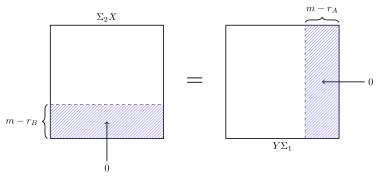
Concretely: the equation for cell $(i,j)$ is trivial if and only if ${\sigma }_i={\tau }_j=0$, that is, $i>r_B$ and $j>r_A$, leaving both entries free (two degrees of freedom); there are $(m-r_B)(m-r_A)$ such cells. Every other cell imposes one non-trivial linear constraint on $(X_{ij},Y_{ij})$, leaving one degree of freedom; there are $m^2-(m-r_A)(m-r_B)$ such cells. The dimensionality of the space of degenerate directions is therefore

$$\begin{array}{rl}& 2(m-r_A)(m-r_B)+\left(m^2-(m-r_A)(m-r_B)\right)\\ & =m^2+(m-r_A)(m-r_B).\end{array}$$

Exercise 2.10 (Redundant units in an MLP). Consider a single-hidden-layer MLP with scalar inputs and outputs, $h$ hidden units with activation function $\sigma :\mathbb{R}\to \mathbb{R}$, and an output bias. The parameter space is $\mathcal{W}={\mathbb{R}}^{3h+1}$ with parameters $w=(a_1,b_1,c_1,\dots ,a_h,b_h,c_h,d)$, and the parameter–function map is

$$f_w(x)=d+\sum _{i=1}^h{a}_i\sigma (b_{i}x+c_i).$$

Here, for each hidden unit $i$, $a_i$ is the outgoing weight, $b_i$ is the incoming weight, and $c_i$ is the bias. The output bias is $d$.

(a) Suppose $a_i=0$ (unit $i$ has zero outgoing weight). Show that the directions $\delta b_i$ and $\delta c_i$ are degenerate at $w$.

(b) Suppose $b_i=0$ (unit $i$ has zero incoming weight). Show that the direction $(\delta a_i,\delta d)=(1,-\sigma (c_i))$ (with all other components zero) is degenerate at $w$.

(c) Suppose $h\ge 2$ and $(b_i,c_i)=(b_j,c_j)$ for some $i\ne j$ (units $i$ and $j$ have the same incoming weights and biases). Show that the direction $(\delta a_i,\delta a_j)=(1,-1)$ (with all other components zero) is degenerate at $w$.

Solution

(a) At $a_i=0$, the parameter–function map reduces to

$$f_w(x)=d+0\cdot \sigma (b_{i}x+c_i)+\sum _{j\ne i}{a}_j\sigma (b_{j}x+c_j)=d+\sum _{j\ne i}{a}_j\sigma (b_{j}x+c_j).$$

This expression does not involve $b_i$ or $c_i$ at all. Therefore $\Phi$ is constant in the $b_i$ and $c_i$ directions at this point, so $D_{\delta b_i}\Phi (w)=0$ and $D_{\delta c_i}\Phi (w)=0$. Both are degenerate directions.

Note that this argument is purely algebraic, following from the multiplicative structure $a_i\cdot \sigma (\dots )$, and requires no conditions on $\sigma$ (not even continuity or differentiability).

(b) At $b_i=0$, unit $i$ computes the constant $\sigma (0\cdot x+c_i)=\sigma (c_i)$ for all $x$, so

$$f_w(x)=d+a_i\sigma (c_i)+\sum _{j\ne i}{a}_j\sigma (b_{j}x+c_j).$$

In the direction $(\delta a_i,\delta d)=(1,-\sigma (c_i))$, we compute

$$\begin{array}{rl}{f}_{w+ϵv}(x)& =(d-ϵ\sigma (c_i))+(a_i+ϵ)\sigma (c_i)+\sum _{j\ne i}{a}_j\sigma (b_{j}x+c_j)\\ & =d+a_i\sigma (c_i)+ϵ(\sigma (c_i)-\sigma (c_i))+\sum _{j\ne i}{a}_j\sigma (b_{j}x+c_j)=f_w(x).\end{array}$$

So $D_{(\delta a_i,\delta d)}\Phi (w)=0$ and this direction is degenerate. Intuitively, increasing $a_i$ scales up the constant contribution $a_i\sigma (c_i)$ to the output, and decreasing $d$ by the same amount compensates exactly.

(c) When $(b_i,c_i)=(b_j,c_j)$, units $i$ and $j$ compute the same activation, so their combined contribution to $f_w$ is

$$a_i\sigma (b_{i}x+c_i)+a_j\sigma (b_{j}x+c_j)=(a_i+a_j)\sigma (b_{i}x+c_i).$$

In the direction $(\delta a_i,\delta a_j)=(1,-1)$, this combined contribution changes by $\sigma (b_{i}x+c_i)-\sigma (b_{j}x+c_j)=0$. All other terms in $f_w$ are unchanged, so $D_{(1,-1)}\Phi (w)=0$. Again, no conditions on $\sigma$ are needed.

2.4 Degeneracy and information singularities

In the preceding sections, we studied degeneracy as a property of parameter–function maps. In the statistical framework introduced in Subsection 1.3, the fundamental object is instead a parameter–distribution map $\Psi :\mathcal{W}\to \mathcal{D}$ ($w\mapsto p_w:\mathcal{X}\to \Delta (\mathcal{Y})$). In this section, we extend the definition of degeneracy to parameter–distribution maps and connect it to a classical quantity from statistics, the Fisher information matrix. We will show that under mild regularity conditions on the statistical model, the Fisher information matrix is singular at $w$ (has zero eigenvalues) if and only if the parameter–distribution map is degenerate at $w$.

Given a parameter–distribution map $\Psi :\mathcal{W}\to \mathcal{D}$, say that $\Psi$ is degenerate at $w$ in direction $v$ if the conditional density does not change to first order:

Here, $D_v\Psi (w)$ is not a conditional distribution but a signed difference between conditional distributions, effectively a real function of $x$ and $y$ (in particular, it may include negative density changes). We mean that this function is zero for all $x\in \mathcal{X}$ and all $y\in \mathcal{Y}$.

Equation 21 extends the definition of degeneracy from Equation 19. If $\Psi$ is constructed from a parameter–function map $\Phi$ via a noise model (as in Subsection 1.3), then degeneracy of $\Phi$ at $w$ in direction $v$ implies degeneracy of $\Psi$ at $w$ in direction $v$, since $p(y\mid x,w)$ depends on $w$ only through $f_w(x)$.

To relate degeneracy to the Fisher information matrix, we introduce two standard definitions.

Definition 2.3 (Score function). Let $\Psi :\mathcal{W}\to \mathcal{D}$ be a parameter–distribution map with densities $p(y\mid x,w)$ that are positive and differentiable in $w$. The score function at $w$ is

$$s(x,y,w)={\nabla }_w\log p(y\mid x,w)\in {\mathbb{R}}^d.$$

The directional score in non-zero direction $v\in {\mathbb{R}}^d$ is

$$s_v(x,y,w)=D_v\log p(y\mid x,w)=\frac{v}{\Vert v\Vert }\cdot {\nabla }_w\log p(y\mid x,w).$$

The directional score measures how sensitive the log-density is to perturbations of $w$ in direction $v$.

Exercise 2.11 (Basic properties of the score function). Let $\Psi :\mathcal{W}\to \mathcal{D}$ be a parameter–distribution map with positive densities $p(y\mid x,w)$, differentiable in $w$. Assume that for each $x$ and $w$, the operations ${\nabla }_w$ and ${\int }_{\mathcal{Y}}\cdot dy$ may be exchanged.

(a) Show that the score function satisfies the following identity: for each $x\in \mathcal{X}$, $y\in \mathcal{Y}$, and $w\in \mathcal{W}$,

$$s(x,y,w)=\frac{{\nabla }_{w}p(y\mid x,w)}{p(y\mid x,w)}.$$

(b) Show that the expected score is zero: for each $x\in \mathcal{X}$ and $w\in \mathcal{W}$,

$${\mathbb{E}}_{y\sim p(y\mid x,w)}[s(x,y,w)]=0.$$

Hint

Differentiate the identity ${\int }_{\mathcal{Y}}p(y\mid x,w)dy=1$.

(c) Show that if $\Psi$ is degenerate at $w$ in direction $v$, then the directional score vanishes identically: $s_v(x,y,w)=0$ for all $x\in \mathcal{X}$ and $y\in \mathcal{Y}$.

(d) Show the converse: if the directional score $s_v(x,y,w)=0$ vanishes for all $x\in \mathcal{X}$ and $y\in \mathcal{Y}$ at $w$, then $\Psi$ is degenerate at $w$ in direction $v$.

Solution

(a) Since $p(y\mid x,w)>0$, the logarithm is well-defined and the chain rule gives

$${\nabla }_w\log p(y\mid x,w)=\frac{{\nabla }_{w}p(y\mid x,w)}{p(y\mid x,w)}.$$

The left-hand side is $s(x,y,w)$ by definition.

(b) Differentiate the normalisation identity ${\int }_{\mathcal{Y}}p(y\mid x,w)dy=1$ with respect to $w$:

$$0={\nabla }_w{\int }_{\mathcal{Y}}p(y\mid x,w)dy={\int }_{\mathcal{Y}}{\nabla }_{w}p(y\mid x,w)dy.$$

By part (a), ${\nabla }_{w}p=p\cdot s$, so

$$0={\int }_{\mathcal{Y}}p(y\mid x,w)s(x,y,w)dy={\mathbb{E}}_{y\sim p(y\mid x,w)}[s(x,y,w)].$$

(c) If $D_v\Psi (w)=0$, then by the definition of degeneracy (21), $D_{v}p(y\mid x,w)=0$ for all $x,y$. By part (a), ${\nabla }_{w}p=p\cdot s$, so contracting both sides with $v/\Vert v\Vert$ gives $D_{v}p=p\cdot s_v$. Since $p>0$, we conclude $s_v(x,y,w)=0$ for all $x,y$.

(d) If $s_v(x,y,w)=0$ for all $x,y$, then by part (a),

$$D_{v}p(y\mid x,w)=p(y\mid x,w)\cdot s_v(x,y,w)=0$$

for all $x,y$ (using $p>0$). That is, $D_v\Psi (w)=0$.

Definition 2.4 (Fisher information matrix). Let $\Psi :\mathcal{W}\to \mathcal{D}$ be a parameter–distribution map with score function $s$. Let $q(x)$ denote the marginal distribution of inputs. The Fisher information matrix $I:\mathcal{W}\to {\mathbb{R}}^{d\times d}$ is defined by

$$I(w)={\mathbb{E}}_{x\sim q(x)}{\mathbb{E}}_{y\sim p(y\mid x,w)}[s(x,y,w)s(x,y,w{)}^{\top }].$$

The Fisher information matrix is symmetric and positive semidefinite at every $w$ (being an expectation of positive semidefinite matrices $s{s}^{\top }$). However, the Fisher information matrix may not be symmetric positive definite, that is, it may be singular.

The following exercise shows that singularity of the Fisher information matrix is equivalent to degeneracy of the parameter–distribution map under mild regularity conditions.

Exercise 2.12 (Fisher information and degeneracy). Let $\Psi :\mathcal{W}\to \mathcal{D}$ be a parameter–distribution map with densities $p(y\mid x,w)$. Assume that $p(y\mid x,w)>0$ for all $y\in \mathcal{Y}$, $x\in \mathcal{X}$, $w\in \mathcal{W}$, that $w\mapsto p(y\mid x,w)$ is differentiable, and that $q(x)>0$ for all $x\in \mathcal{X}$.

(a) Show that for any unit vector $v\in {\mathbb{R}}^d$,

$$v^{\top }I(w)v={\mathbb{E}}_{x\sim q(x)}{\mathbb{E}}_{y\sim p(y\mid x,w)}[s_v(x,y,w{)}^2].$$

(b) Using Exercise 2.11(c), show that if $D_v\Psi (w)=0$ for some non-zero $v$, then $I(w)$ is not positive definite.

Hint

Check the definition of positive definite.

(c) Using Exercise 2.11(d), show that if $I(w)$ is not positive definite, then there exists a non-zero $v$ for which $D_v\Psi (w)=0$.

Hint

Check the definition of positive definite.

(d) Conclude that

$$\ker I(w)=\{v\in {\mathbb{R}}^d:D_v\Psi (w)=0\}.$$

That is, the null space of the Fisher information matrix is exactly the space of degenerate directions of the parameter–distribution map.

Solution

(a) Since $v$ is a unit vector, $s_v=D_v\log p=\frac{v}{\Vert v\Vert }\cdot s=v\cdot s$. From the definition of $I(w)$ in (26),

$$\begin{array}{rl}{v}^{\top }I(w)v& =v^{\top }{\mathbb{E}}_{x,y}\left[s{s}^{\top }\right]v={\mathbb{E}}_{x,y}[(v\cdot s{)}^2]={\mathbb{E}}_{x,y}[s_v^2]\\ & ={\mathbb{E}}_{x\sim q(x)}{\mathbb{E}}_{y\sim p(y\mid x,w)}[s_v(x,y,w{)}^2].\end{array}$$

(b) If $D_v\Psi (w)=0$ for some non-zero $v$, then by Exercise 2.11(c), $s_v(x,y,w)=0$ for all $x,y$. Let $\hat{v}=v/\Vert v\Vert$. Then $s_{\hat{v}}=s_v$ (the directional derivative is invariant to the magnitude of $v$), so by part (a), ${\hat{v}}^{\top }I(w)\hat{v}=\mathbb{E}[s_{\hat{v}}^2]=0$. A matrix $M$ is positive definite only if $u^{\top }Mu>0$ for all non-zero $u$. Since $\hat{v}$ is a non-zero vector with ${\hat{v}}^{\top }I(w)\hat{v}=0$, the matrix $I(w)$ is not positive definite.

(c) If $I(w)$ is not positive definite, then since $I(w)$ is positive semidefinite, there exists a non-zero vector $\hat{v}$ such that ${\hat{v}}^{\top }I(w)\hat{v}=0$. By part (a) (taking $\hat{v}$ to be a unit vector without loss of generality), $\mathbb{E}[s_{\hat{v}}^2]=0$. Since $s_{\hat{v}}^2\ge 0$ and $q(x)>0$ and $p(y\mid x,w)>0$, this implies $s_{\hat{v}}(x,y,w)=0$ for all $x\in \mathcal{X}$ and $y\in \mathcal{Y}$. By Exercise 2.11(d), $D_{\hat{v}}\Psi (w)=0$.

(d) Parts (b) and (c) show that $I(w)$ is positive definite if and only if $\Psi$ is non-degenerate at $w$, or equivalently, $I(w)$ is singular if and only if $\Psi$ is degenerate at $w$.

For the kernel characterisation: clearly $0\in \ker I(w)$. For non-zero $v$, $v\in \ker I(w)$ means $I(w)v=0$, which (since $I(w)$ is positive semidefinite) is equivalent to $v^{\top }I(w)v=0$. Normalising to $\hat{v}=v/\Vert v\Vert$, part (a) gives $\mathbb{E}[s_{\hat{v}}^2]=0$, which as in part (c) implies $s_{\hat{v}}=0$ everywhere. By Exercise 2.11(d), $D_{\hat{v}}\Psi (w)=0$, and hence $D_v\Psi (w)=0$. Conversely, if $D_v\Psi (w)=0$ for non-zero $v$, then Exercise 2.11(c) gives $s_v=0$, so $v^{\top }I(w)v=\Vert v{\Vert }^2\mathbb{E}[s_v^2]=0$, hence $I(w)v=0$. Therefore $\ker I(w)=\{v\in {\mathbb{R}}^d:D_v\Psi (w)=0\}$.

2.5 Degeneracy and the loss landscape

In the preceding sections, we studied degeneracy as a property of parameter–function maps and parameter–distribution maps. We now consider the implications of degeneracy in these maps for the loss landscape in which deep learning algorithms operate.

Recall the definitions of loss functions from Section 1. In what follows, we assume that the per-example loss $L_{x,y}(w)$ depends on $w$ only through $\Phi (w)$, and work with the population loss $L(w)={\mathbb{E}}_{(x,y)\sim q}[L_{x,y}(w)]$. For statistical models, we use the expected negative log likelihood $L(w)={\mathbb{E}}_{(x,y)\sim q}[-\log p(y\mid x,w)]$ as our loss function. In either case, we assume that $L$ is twice-differentiable with respect to $w$.

Let us begin with some basic observations about the relationship between degeneracy in parameter–function maps and directional derivatives in the loss landscape.

Exercise 2.13 (Directional derivatives of the loss). Let $L:\mathcal{W}\to \mathbb{R}$ be a population loss function satisfying the assumptions described above.

(a) Show that if $\Phi$ is degenerate at $w$ in direction $v$, then the directional derivative of the loss vanishes in the same direction: $D_{v}L(w)=0$.

(b) Suppose $\mathcal{W}={\mathbb{R}}^d$. Show that if $d>1$, then for any $w\in \mathcal{W}$, there exists a nonzero $v$ such that $D_{v}L(w)=0$.

Hint

consider separately the cases $\nabla L(w)=0$ and $\nabla L(w)\ne 0$.

Solution

(a) Since $L_{x,y}(w)$ depends on $w$ only through $\Phi (w)$, we can write $L_{x,y}(w)={\ell }_{x,y}(\Phi (w))$ for some functional ${\ell }_{x,y}$. If $D_v\Phi (w)=0$, then $\Phi (w+ϵv)=\Phi (w)+O({ϵ}^2)$ as $ϵ\to 0$, and therefore $L_{x,y}(w+ϵv)={\ell }_{x,y}(\Phi (w)+O({ϵ}^2))=L_{x,y}(w)+O({ϵ}^2)$. Taking expectations over $(x,y)\sim q$,

$$L(w+ϵv)=L(w)+O({ϵ}^2),$$

so $D_{v}L(w)={\lim }_{ϵ\to 0}\frac{L(w+ϵv)-L(w)}{ϵ\Vert v\Vert }=0$.

(b) If $\nabla L(w)=0$, then $D_{v}L(w)=\frac{v}{\Vert v\Vert }\cdot \nabla L(w)=0$ for every nonzero $v$.

If $\nabla L(w)\ne 0$, the orthogonal complement $\nabla L(w{)}^{\perp }$ has dimension $d-1\ge 1$ (since $d>1$). Pick any nonzero $v\in \nabla L(w{)}^{\perp }$. Then $D_{v}L(w)=\frac{v}{\Vert v\Vert }\cdot \nabla L(w)=0$.

We see that parameter–function map degeneracy implies flat loss directions, but a vanishing directional derivative of the loss landscape is commonplace. To find a satisfying definition of degeneracy in a loss landscape, we must look at second-order information.

Define the Hessian matrix $H(w)\in {\mathbb{R}}^{d\times d}$ of the loss at $w$ by

$$H(w{)}_{jk}=\frac{{\partial }^{2}L}{\partial w_j\partial w_k}(w).$$

The Hessian at $w$ is sometimes denoted ${\nabla }^{2}L(w)$. The Hessian captures the local curvature of the loss landscape via the quadratic approximation

$$L(w+\delta )\approx L(w)+\nabla L(w{)}^{\top }\delta +\frac{1}{2}{\delta }^{\top }H(w)\delta .$$

At a critical point ($\nabla L(w)=0$), the Hessian determines whether the loss curves upward, downward, or remains flat in each direction.

In particular, at a local minimum, $H(w)$ is positive semidefinite. We can therefore classify local minima as follows:

• A local minimum $w$ is regular (or non-degenerate, or Morse) if $H(w)$ is positive definite.
• A local minimum $w$ is degenerate (or non-Morse) if $H(w)$ is singular (has a zero eigenvalue).

Exercise 2.14 (Some examples of loss landscape degeneracy). Consider the parameter space $\mathcal{W}={\mathbb{R}}^2$ with the identity parameter–function map $\Phi =\mathrm{id}$, so that we identify parameters with the functions they implement (cf., Exercise 2.1). Consider the family of loss functions $L_{k,l}(a,b)=a^{2k}+b^{2l}$ for non-negative integers $k$ and $l$.

(a) Show that the origin is a global minimum of $L_{k,l}$ for all non-negative $k$ and $l$. For which $k$ and $l$ is it the unique global minimum?

(b) Show that if $k=l=1$, then the origin is a non-degenerate (regular) minimum.

Hint

Compute the Hessian.

(c) Show that if $k>1$ and $l\ge 1$, then the origin is a degenerate minimum.

(d) Show that if $k=0$ and $l\ge 1$, then the origin is a degenerate minimum.

Solution

(a) Since $a^{2k}\ge 0$ and $b^{2l}\ge 0$ for all $a,b\in \mathbb{R}$ (using the convention $0^0=1$), we have $L_{k,l}(a,b)\ge 0$ for $k,l\ge 1$, $L_{k,l}(a,b)\ge 1$ if $k=0$ or $l=0$, and $L_{k,l}(a,b)=2$ if $k=l=0$. At the origin, $L_{k,l}(0,0)=0^{2k}+0^{2l}$, which equals $0$ if $k\ge 1$ and $l\ge 1$, equals $1$ if exactly one of $k,l$ is $0$, and equals $2$ if $k=l=0$. In each case this matches the lower bound, so the origin is a global minimum.

The origin is the unique global minimum if and only if $k\ge 1$ and $l\ge 1$: then $L_{k,l}(a,b)=0$ requires both $a^{2k}=0$ and $b^{2l}=0$, forcing $a=b=0$. If $k=0$, then $L_{0,l}(a,0)=1$ for all $a$, so the entire $a$-axis achieves the minimum. Similarly if $l=0$. If $k=l=0$, then all parameters achieve the minimum.

(b) For $k=l=1$: $L_{1,1}(a,b)=a^2+b^2$. The Hessian at the origin is

$$H(0,0)=\left(\begin{array}{cc}2& 0\\ 0& 2\end{array}\right),$$

which is positive definite. The origin is a non-degenerate minimum.

(c) For $k>1$ and $l\ge 1$: $\frac{{\partial }^2{L}_{k,l}}{\partial a^2}=2k(2k-1)a^{2k-2}$. At the origin, $a^{2k-2}=0$ since $2k-2\ge 2$, so this entry vanishes. The Hessian at the origin is therefore

$$H(0,0)=\left(\begin{array}{cc}0& 0\\ 0& 2l(2l-1)\cdot 0^{2l-2}\end{array}\right),$$

which has a zero eigenvalue (from the first diagonal entry) regardless of the value of the second. The origin is a degenerate minimum.

(d) For $k=0$ and $l\ge 1$: $L_{0,l}(a,b)=1+b^{2l}$. Since $L_{0,l}$ is independent of $a$, both $\frac{\partial L}{\partial a}$ and $\frac{{\partial }^{2}L}{\partial a^2}$ vanish identically. The Hessian at the origin has a zero first diagonal entry, so it is singular. The origin is a degenerate minimum.

Note that the Hessian degeneracy in Exercise 2.14(c) and 2.14(d) arise for qualitatively different reasons. In Exercise 2.14(d), the loss is constant along the $a$-direction to all orders—a genuinely flat direction. In Exercise 2.14(c), the loss does increase along the $a$-direction, just more slowly than quadratically (as $a^4$, $a^6$, etc., depending on $k$). Moreover, different values of $k$ give different rates of increase. The Hessian cannot distinguish any of these cases: flat, quartic, and so on all appear the same from the perspective of the Hessian rank. We will later see approaches that can distinguish these degrees of degeneracy.

So much for defining loss landscape degeneracy. What is the relationship between this kind of degeneracy and degeneracy of the parameter–function/distribution map?

The relationship is subtle, and generally depends on the choice of loss function. One natural setting in which to study this relationship is the realisable statistical model: given a parameter–distribution map and a parameter $w_0$, if we consider $p_{w_0}$ as the true data-generating distribution, the population negative log-likelihood loss will have a global minimum at $w_0$. The following exercise shows that in this setting, under mild regularity assumptions on the statistical model, degeneracy in the parameter–distribution map at $w_0$ implies that the global minimum $w_0$ is a degenerate global minimum of the loss landscape.

Exercise 2.15 (Realisable models and Hessian degeneracy). Let $\Psi :\mathcal{W}\to \mathcal{D}$ be a parameter–distribution map with positive densities $p(y\mid x,w)$, twice-differentiable in $w$. Suppose data is generated from a fixed true parameter $w_0\in \mathcal{W}$, meaning $q(y\mid x)=p(y\mid x,w_0)$. Consider the population negative log-likelihood loss

$$L(w)=-{\mathbb{E}}_{x\sim q(x)}{\mathbb{E}}_{y\sim p(y\mid x,w_0)}[\log p(y\mid x,w)].$$

Assume that for each $x$, the operations ${\nabla }_w$ (and ${\nabla }_w^2$) and ${\int }_{\mathcal{Y}}\cdot dy$ may be exchanged.

(a) (Bartlett identity.) Show that for each $x\in \mathcal{X}$ and $w\in \mathcal{W}$,

$$-{\mathbb{E}}_{y\sim p(y\mid x,w)}[{\nabla }_w^2\log p(y\mid x,w)]={\mathbb{E}}_{y\sim p(y\mid x,w)}[s(x,y,w)s(x,y,w{)}^{\top }],$$

where $s$ is the score function from Definition 2.3.

Hint

differentiate the identity ${\mathbb{E}}_{y\sim p(y\mid x,w)}[s(x,y,w)]=0$ (established in Exercise 2.11) with respect to $w$.

(b) Show that the Hessian of $L$ at the true parameter $w_0$ equals the Fisher information matrix (Definition 2.4):

$$H(w_0)=I(w_0).$$

Hint

compute $H(w)=-{\mathbb{E}}_x{\mathbb{E}}_{y\sim p(y\mid x,w_0)}[{\nabla }_w^2\log p(y\mid x,w)]$, evaluate at $w=w_0$, and apply part (a).

(c) Using the result of Exercise 2.12, conclude: if $\Psi$ is degenerate at $w_0$ in direction $v$, then $H(w_0)v=0$. Contrapositively, if $H(w_0)$ is positive definite, then $\Psi$ is non-degenerate at $w_0$.

Solution

(a) From Exercise 2.11, ${\mathbb{E}}_{y\sim p(y\mid x,w)}[s_j(x,y,w)]=0$ for each component $j$ of the score, where $s_j=\frac{\partial }{\partial w_j}\log p(y\mid x,w)$. Differentiating with respect to $w_k$ and exchanging the derivative with the integral:

$$\begin{array}{rl}0& =\frac{\partial }{\partial w_k}{\int }_{\mathcal{Y}}{s}_j(x,y,w)p(y\mid x,w)dy\\ & ={\int }_{\mathcal{Y}}\frac{\partial s_j}{\partial w_k}pdy+{\int }_{\mathcal{Y}}{s}_j\frac{\partial p}{\partial w_k}dy.\text{(product rule)}\end{array}$$

Using the score identity $\frac{\partial p}{\partial w_k}=p\cdot s_k$ (24), the second integral becomes ${\int }_{\mathcal{Y}}{s}_j{s}_{k}pdy={\mathbb{E}}_y[s_j{s}_k]$. Therefore

$${\mathbb{E}}_{y\sim p(y\mid x,w)}\left[\frac{{\partial }^2\log p}{\partial w_j\partial w_k}\right]=-{\mathbb{E}}_{y\sim p(y\mid x,w)}[s_j{s}_k].$$

Assembling all components into a matrix gives

$$-{\mathbb{E}}_{y\sim p(y\mid x,w)}[{\nabla }_w^2\log p(y\mid x,w)]={\mathbb{E}}_{y\sim p(y\mid x,w)}[s(x,y,w)s(x,y,w{)}^{\top }].$$

(b) The population negative log-likelihood is $L(w)=-{\mathbb{E}}_{x\sim q(x)}{\mathbb{E}}_{y\sim p(y\mid x,w_0)}[\log p(y\mid x,w)]$. Taking the Hessian with respect to $w$ (exchanging differentiation and integration):

$$H(w)=-{\mathbb{E}}_{x\sim q(x)}{\mathbb{E}}_{y\sim p(y\mid x,w_0)}[{\nabla }_w^2\log p(y\mid x,w)].$$

At $w=w_0$, the inner expectation is over $y\sim p(y\mid x,w_0)$, which matches the distribution in the Bartlett identity. Applying part (a):

$$\begin{array}{rl}H(w_0)& ={\mathbb{E}}_{x\sim q(x)}{\mathbb{E}}_{y\sim p(y\mid x,w_0)}[s(x,y,w_0)s(x,y,w_0{)}^{\top }]\\ & =I(w_0).\text{(by Definition 2.4)}\end{array}$$

(c) By Exercise 2.12, $\ker I(w_0)=\{v\in {\mathbb{R}}^d:D_v\Psi (w_0)=0\}$. Since $H(w_0)=I(w_0)$, if $\Psi$ is degenerate at $w_0$ in direction $v$, then $v\in \ker I(w_0)=\ker H(w_0)$, so $H(w_0)v=0$.

Contrapositively: if $H(w_0)$ is positive definite, then $\ker H(w_0)=\{0\}$, so $\ker I(w_0)=\{0\}$, and $\Psi$ is non-degenerate at $w_0$.

Exercise 2.15 shows that for the population negative log-likelihood at the true parameter, degeneracy of the parameter–distribution map implies a degenerate loss landscape. The converse does not hold in general, nor does the forward direction hold at arbitrary points in parameter space. The following exercise explores these subtleties through examples.

Exercise 2.16 (Contrasting parametric versus loss degeneracy). (a) Observe that the identity parameter–function map on $\mathcal{W}={\mathbb{R}}^2$ is non-degenerate everywhere. With this in mind, what do your answers to Exercise 2.14(b), 2.14(c) and 2.14(d) exemplify about the logical relationship between parameter–function map degeneracy and loss landscape degeneracy?

(b) Consider again the identity parameter–function map on $\mathcal{W}={\mathbb{R}}^2$. Consider the loss function $L_{\circ }(a,b)=(a^2+b^2-1{)}^2$. Find a global minimum of $L_{\circ }$ and show that it is a degenerate critical point. What does this example reveal about the logical relationship between parameter–function map degeneracy and loss landscape degeneracy?

(c) Now consider the cubic parameter–function map $\Phi (\alpha ,\beta )=({\alpha }^3,{\beta }^3)$.

1. Argue that $\Phi$ is degenerate at the origin (cf., Exercise 2.2).
2. If we take $L_{k,l}$ from Exercise 2.14 to be defined on the constant function $(a,b)$ (rather than equivalent underlying parameter), then in this parameterisation, that loss function becomes $L_{k,l}(\alpha ,\beta )=({\alpha }^3{)}^{2k}+({\beta }^3{)}^{2l}$. Show that the origin is a degenerate minimum of $L_{k,l}$ for all $k\ge 0$ and $l\ge 0$ under this parametrisation.
3. What does this example reveal about the logical relationship between parameter–function map degeneracy and loss landscape degeneracy?

(d) Consider the product parameter–function map $\Phi (a,b)=a\cdot b$ from Exercise 2.3, and define $L(a,b)=\frac{1}{2}(ab-1{)}^2$.

1. Show that $(0,0)$ is a critical point and that $\Phi$ is degenerate in every direction at $(0,0)$.
2. Compute the Hessian at $(0,0)$ and show it is nonsingular.
3. What does this example reveal about the logical relationship between parameter–function map degeneracy and loss landscape degeneracy? Why does this not contradict Exercise 2.15?

Solution

(a) The identity parameter–function map $\Phi (a,b)=(a,b)$ has Jacobian equal to the $2\times 2$ identity matrix everywhere, so it is non-degenerate at every point. Exercise 2.14(b) shows that $L_{1,1}$ has a non-degenerate minimum: absence of parameter–function map degeneracy is consistent with absence of loss landscape degeneracy. Exercise 2.14(c) and 2.14(d) show that $L_{2,1}$, $L_{0,1}$, etc., have degenerate minima despite the parameter–function map being non-degenerate. This demonstrates that loss landscape degeneracy does not imply parameter–function map degeneracy.

(b) $L_{\circ }(a,b)=(a^2+b^2-1{)}^2\ge 0$, with equality if and only if $a^2+b^2=1$. So every point on the unit circle is a global minimum. Consider $(1,0)$. The gradient is

$$\nabla L_{\circ }=(4a(a^2+b^2-1),4b(a^2+b^2-1)),$$

which vanishes at $(1,0)$. The Hessian entries at $(1,0)$ are:

$$\begin{array}{rlrl}\frac{{\partial }^2{L}_{\circ }}{\partial a^2}& =4(3a^2+b^2-1)=8,& \frac{{\partial }^2{L}_{\circ }}{\partial b^2}& =4(a^2+3b^2-1)=0,\\ \frac{{\partial }^2{L}_{\circ }}{\partial a\partial b}& =8ab=0.& & \end{array}$$

So $H(1,0)=\mathrm{diag}(8,0)$, which is singular. Therefore, $(1,0)$ is a degenerate minimum.

This provides another example of loss landscape degeneracy without parameter–function map degeneracy: the identity parameter–function map is non-degenerate, but the circle of global minima creates a flat tangential direction.

(c)

1. The map $\Phi (\alpha ,\beta )=({\alpha }^3,{\beta }^3)$ is the product of two copies of the cubic parametrisation from Exercise 2.2. In each component, the derivative $\frac{d}{d\alpha }({\alpha }^3)=3{\alpha }^2$ vanishes at $\alpha =0$. Therefore both coordinate directions are degenerate at the origin, and hence every direction is degenerate at the origin (since the Jacobian $\mathrm{diag}(3{\alpha }^2,3{\beta }^2)$ is the zero matrix there).
2. In the new parametrisation, the loss becomes $L_{k,l}(\alpha ,\beta )=({\alpha }^3{)}^{2k}+({\beta }^3{)}^{2l}={\alpha }^{6k}+{\beta }^{6l}$.

If $k\ge 1$ and $l\ge 1$: the exponents $6k$ and $6l$ are both at least $6$, so $\frac{{\partial }^{2}L}{\partial {\alpha }^2}{|}_0=6k(6k-1)\cdot 0^{6k-2}=0$ (since $6k-2\ge 4$), and similarly for $\beta$. The Hessian at the origin is the zero matrix, which is singular.

If $k=0$: $L_{0,l}(\alpha ,\beta )=1+{\beta }^{6l}$, which is independent of $\alpha$, so the Hessian has a zero first diagonal entry. Similarly if $l=0$. In all cases, the origin is a degenerate minimum. 3. Under the identity parameter–function map, $L_{1,1}(a,b)=a^2+b^2$ had a non-degenerate minimum at the origin (Exercise 2.14(b)). Under the cubic parameter–function map, the same loss became ${\alpha }^6+{\beta }^6$, which has a degenerate minimum at the origin. This shows that introducing degeneracy into the parameter–function map can convert a non-degenerate minimum into a degenerate one.

For other $k,l$, $L_{k,l}$ was already degenerate at the origin under the non-degenerate parameterisation, the cubic function only makes it more degenerate (in terms of the order to which the loss vanishes in the degenerate direction(s); we will formally quantify this in Section 3).

(d)

1. The gradient is $\nabla L=(ab-1)(b,a)$. At $(0,0)$: $\nabla L=(0-1)(0,0)=(0,0)$. So $(0,0)$ is a critical point.

The Jacobian of $\Phi (a,b)=ab$ is $(b,a)$, which at $(0,0)$ is $(0,0)$. Every direction $v=(v_1,v_2)$ gives $Jv=b{v}_1+a{v}_2=0$, so $\Phi$ is degenerate in every direction at $(0,0)$. 2. Computing second partial derivatives:

$$\begin{array}{rlrlrl}\frac{{\partial }^{2}L}{\partial a^2}& =b^2,& \frac{{\partial }^{2}L}{\partial b^2}& =a^2,& \frac{{\partial }^{2}L}{\partial a\partial b}& =2ab-1.\end{array}$$

At $(0,0)$:

$$H(0,0)=\left(\begin{array}{cc}0& -1\\ -1& 0\end{array}\right),$$

which has determinant $-1\ne 0$ (eigenvalues $\pm 1$). The Hessian is nonsingular. 3. Despite full degeneracy of the parameter–function map at $(0,0)$, the Hessian is nonsingular (in fact indefinite, so $(0,0)$ is a saddle point, not a local minimum). This shows that parameter–function map degeneracy does not in general imply loss landscape degeneracy.

This does not contradict Exercise 2.15, which establishes $H(w_0)=I(w_0)$ at the true parameter $w_0$, meaning $\Phi (w_0)$ must equal the target. Here, $\Phi (0,0)=0\ne 1$, so $(0,0)$ is not the true parameter, and the identity does not apply.

3. The degeneracy hierarchy

We have so far explored different kinds of qualitative degeneracy in the loss landscape. A natural question arises: how can we quantify the degree of degeneracy at a particular point in parameter space? In this section, we introduce the local learning coefficient, a rich mathematical object that reflects the degree of degeneracy at a parameter, and we explore it from several perspectives.

In this section and Section 4 we assume that any population loss $L$ is a real analytic function. The precise definition of real analyticity is not important for this tutorial but interested readers can refer to (Watanabe 2009) (section 2). A property that will be useful is that such functions have a convergent Taylor expansion, in particular they have smooth derivatives of all orders.

3.1 The local learning coefficient via volume scaling asymptotics

The key idea is to measure the volume of near-optimal parameters. Consider a local minimum $w^{\ast }\in \mathcal{W}$ of the population loss $L$, and suppose we have a sufficiently small closed ball $B(w^{\ast })$ centred on $w^{\ast }$ such that $L(w)\ge L(w^{\ast })$ for all $w\in B(w^{\ast })$. Given a tolerance $ϵ>0$, define the sublevel set

consisting of all parameters in the ball whose loss is within $ϵ$ of the minimum. The volume of this set is

$$V(ϵ):=\mathrm{Vol}(B(w^{\ast },ϵ))={\int }_{B(w^{\ast },ϵ)}dw.$$

We will look at how this volume scales as $ϵ\to 0$. It will be instructive for us to first calculate this scaling in the non-degenerate case.

Exercise 3.1 (Volume scaling in the regular case). Let $w^{\ast }\in \mathcal{W}$ be a local minimum of $L$, and suppose that the Hessian ${\nabla }^{2}L(w^{\ast })$ is positive definite. Show that

$$V(ϵ)=c{ϵ}^{d/2}+o({ϵ}^{d/2})\text{as }ϵ\to 0,$$

for some constant $c>0$ where $d=\dim (\mathcal{W})$. You may assume that, as $ϵ\to 0$, the volume of $B(w^{\ast },ϵ)$ agrees to leading order with the volume of the quadratic approximation obtained by replacing $L$ with its second-order Taylor expansion at $w^{\ast }$.

Hint

The volume of the ellipsoid $\{\mathbf{x}\in {\mathbb{R}}^d\mid {\mathbf{x}}^{\top }A\mathbf{x}<1\}$ is proportional to $(\det A{)}^{-1/2}$.

Solution

Because $w^{\ast }$ is a local minimum, the gradient $\nabla L(w^{\ast })$ is zero. By Taylor's theorem, we can write the loss function near $w^{\ast }$ exactly as:

$$L(w)-L(w^{\ast })=\frac{1}{2}(w-w^{\ast }{)}^{\top }H(w-w^{\ast })+o(\Vert w-w^{\ast }{\Vert }^2)$$

where $H={\nabla }^{2}L(w^{\ast })$ is the strictly positive definite Hessian matrix.

The sublevel set is defined by the condition $L(w)-L(w^{\ast })<ϵ$. As $ϵ\to 0$, the neighborhood of parameters that satisfy this condition shrinks toward $w^{\ast }$. In this limit, the higher-order error term $o(\Vert w-w^{\ast }{\Vert }^2)$ becomes negligible, and the boundary of the sublevel set is governed entirely by the quadratic form:

$$\frac{1}{2}(w-w^{\ast }{)}^{\top }H(w-w^{\ast })<ϵ.$$

We can rewrite this inequality into the standard form of an ellipsoid, $x^{\top }Ax<1$, by dividing both sides by $ϵ$:

$$(w-w^{\ast }{)}^{\top }\left(\frac{1}{2ϵ}H\right)(w-w^{\ast })<1.$$

Using the hint, the volume of a $d$-dimensional ellipsoid defined by a matrix $A$ is proportional to $(\det A{)}^{-1/2}$. Here, our matrix is $A=\frac{1}{2ϵ}H$.

Therefore,

$$\det {\left(\frac{1}{2ϵ}H\right)}^{-1/2}={\left({\left(\frac{1}{2ϵ}\right)}^d\det H\right)}^{-1/2}={ϵ}^{d/2}\underset{:=c}{\underbrace{{\left(\frac{\det H}{2^d}\right)}^{-1/2}}}$$

Because the true loss function deviates from this pure quadratic form only by an error of $o(\Vert w-w^{\ast }{\Vert }^2)$, the volume of the true sublevel set deviates from the ellipsoid's volume only by a correspondingly higher-order error term. Thus, we conclude:

$$V(ϵ)=c{ϵ}^{d/2}+o({ϵ}^{d/2})\text{as }ϵ\to 0.$$

The key takeaway from this exercise is that the dimension of the model controls the leading order asymptotics of the volume scaling. We can investigate this further by calculating the volume scaling in an example where the Hessian is not positive definite.

Exercise 3.2 (Quadratic Valley Volume Scaling). Let $\mathcal{W}=[-R,R{]}^d$ for some (large) $R\in \mathbb{R}$ and let $L(x_1,\dots ,x_d)=\sum _{i=1}^{d^{\prime }}{x}_i^2$.

(a) Sketch the loss landscape when $d=2,d^{\prime }=1$.

(b) $L$ achieves its minimum value $0$ at multiple points in $\mathcal{W}$. What is the dimension of the space ${\mathcal{W}}_0:=\{w\in \mathcal{W}|L(w)=0\}$?

(c) Calculate the Hessian of $L$.

(d) Prove that $V(ϵ)\propto {ϵ}^{d^{\prime }/2}$

Hint

Use the volume of the ellipsoid from Exercise 3.1

Solution

(a) The loss is $L(x_1,x_2)=x_1^2$, which is a parabolic trough: a parabola in the $x_1$ direction and constant along $x_2$. The zero set is the line $x_1=0$.

(b) ${\mathcal{W}}_0=\{0{\}}^{d^{\prime }}\times [-R,R{]}^{d-d^{\prime }}$, which is a $(d-d^{\prime })$-dimensional affine subspace of $\mathcal{W}$. Hence $\dim ({\mathcal{W}}_0)=d-d^{\prime }$.

(c) Since $L(w)={\sum }_{i=1}^{d^{\prime }}{x}_i^2$, the partial derivatives are

$$\frac{\partial L}{\partial x_i}=\{\begin{array}{ll}2x_i& i\le d^{\prime },\\ 0& i>d^{\prime },\end{array}\frac{{\partial }^{2}L}{\partial x_i\partial x_j}=\{\begin{array}{ll}2& i=j\le d^{\prime },\\ 0& \text{otherwise}.\end{array}$$

So the Hessian is the block diagonal matrix:

$${\nabla }^{2}L=\left(\begin{array}{cc}2I_{d^{\prime }}& 0\\ 0& 0_{d-d^{\prime }}\end{array}\right),$$

which has rank $d^{\prime }$. In particular it is positive semi-definite but not positive definite whenever $d^{\prime }<d$.

(d) The minimum of $L$ is $0$, achieved on ${\mathcal{W}}_0$. For any $w^{\ast }\in {\mathcal{W}}_0$ and $ϵ>0$, the sublevel set is

$$\begin{array}{rl}B(w^{\ast },ϵ)& =\left\{(x_1,\dots ,x_d)\in [-R,R{]}^d|\sum _{i=1}^{d^{\prime }}{x}_i^2<ϵ\right\}\\ & =\left\{x\in {\mathbb{R}}^{d^{\prime }}:\sum _{i=1}^{d^{\prime }}{x}_i^2<ϵ\right\}\times [-R,R{]}^{d-d^{\prime }}\end{array}$$

for $R$ sufficiently large (specifically $\sqrt{ϵ}<R$). The condition ${\sum }_{i=1}^{d^{\prime }}{x}_i^2<ϵ$ can be rewritten as ${\mathbf{x}}^{\top }A\mathbf{x}<1$ where $A={ϵ}^{-1}{I}_{d^{\prime }}$. By the ellipsoid volume formula from Exercise 3.1, the volume of this region is proportional to $(\det A{)}^{-1/2}=({ϵ}^{-d^{\prime }}{)}^{-1/2}={ϵ}^{d^{\prime }/2}$. Multiplying by the volume $(2R{)}^{d-d^{\prime }}$ of the remaining coordinates gives $V(ϵ)\propto {ϵ}^{d^{\prime }/2}$.

In this example, the degenerate directions do not contribute to the leading exponent of $V(ϵ)$. We see that the exponent $\frac{d}{2}$ from Exercise 3.1 is replaced with $\frac{d^{\prime }}{2}$ where $d^{\prime }$ is the codimension of ${\mathcal{W}}_0$ i.e. the effective dimension of $L$ which ignores the degenerate directions. This suggests that we can capture information about the degree of degeneracy of a loss function by looking at how the volume $V(ϵ)$ scales as $ϵ\to 0$. (Watanabe 2009) proves a general form for this kind of volume scaling which has been adapted by (Lau et al. 2025) into the following definition.

Definition 3.1 (Local learning coefficient). Let $w^{\ast }\in \mathcal{W}$ be a local minimum of the population loss $L$. There exists a unique rational number $\lambda (w^{\ast })>0$, a positive integer $\mu (w^{\ast })$, and a constant $c>0$ such that as $ϵ\to 0$,

$$V(ϵ)=c{ϵ}^{\lambda (w^{\ast })}(-\log ϵ{)}^{\mu (w^{\ast })-1}+o\left({ϵ}^{\lambda (w^{\ast })}(-\log ϵ{)}^{\mu (w^{\ast })-1}\right).$$

We call $\lambda (w^{\ast })$ the local learning coefficient (LLC) at $w^{\ast }$, and $\mu (w^{\ast })$ the local multiplicity.

Exercise 3.3 (Two equations for $\lambda$). (a) Prove that for $a>1$

$$\lambda =\underset{ϵ\to 0}{\lim }\frac{\log (V(aϵ)/V(ϵ))}{\log (a)}$$

(b) Prove that

$$\lambda =\underset{ϵ\to 0}{\lim }\frac{\log V(ϵ)}{\log ϵ}$$

Solution

(a) From Definition 3.1, as $ϵ\to 0$,

$$V(ϵ)=c{ϵ}^{\lambda }(-\log ϵ{)}^{m-1}(1+o(1)).$$

Substituting $ϵ\mapsto aϵ$,

$$V(aϵ)=c(aϵ{)}^{\lambda }(-\log (aϵ){)}^{m-1}(1+o(1)).$$

Taking the ratio,

$$\frac{V(aϵ)}{V(ϵ)}=a^{\lambda }{\left(\frac{-\log (aϵ)}{-\log ϵ}\right)}^{m-1}(1+o(1)).$$

As $ϵ\to 0$, $-\log ϵ\to \infty$, and

$$\frac{-\log (aϵ)}{-\log ϵ}=\frac{-\log a-\log ϵ}{-\log ϵ}=1+\frac{\log a}{-\log ϵ}\stackrel{ϵ\to 0}{\to }1.$$

Therefore $V(aϵ)/V(ϵ)\to a^{\lambda }$. Taking logarithms and dividing by $\log a>0$ gives the result.

(b) From Definition 3.1, $V(ϵ)=c{ϵ}^{\lambda (w^{\ast })}(-\log ϵ{)}^{\mu (w^{\ast })-1}(1+o(1))$, so

$$\log V(ϵ)=\lambda (w^{\ast })\log ϵ+(\mu (w^{\ast })-1)\log (-\log ϵ)+\log c+o(1).$$

Dividing by $\log ϵ$

$$\frac{\log V(ϵ)}{\log ϵ}=\lambda (w^{\ast })+\frac{(\mu (w^{\ast })-1)\log (-\log ϵ)}{\log ϵ}+\frac{\log c+o(1)}{\log ϵ}.$$

It remains to prove that the final two terms in this sum vanish as $ϵ\to 0$. The final term tends to $0$ since $\log ϵ\to -\infty$ and the numerator is bounded as $ϵ\to 0$. Now we look at the middle term which is proportional to

$$\underset{ϵ\to 0}{\lim }\frac{\log (-\log ϵ)}{\log ϵ}=\underset{x\to \infty }{\lim }\frac{\log (x)}{-x}=0,$$

completing the proof.

Note that from equation (36) we already have that the LLC and local multiplicity in the regular case are $\lambda =\frac{d}{2}$, $\mu =1$

When $\mu (w^{\ast })=1$, the formula simplifies to $V(ϵ)=c{ϵ}^{\lambda (w^{\ast })}+o({ϵ}^{\lambda (w^{\ast })})$ which allows us to interpret $\lambda (w^{\ast })$ as the volume scaling exponent: increasing the error tolerance by a factor of $a$ increases the volume of near-optimal parameters by a factor of $a^{\lambda (w^{\ast })}$.

Exercise 3.4 (Calculating the LLC). Calculate the LLC and the rank of the Hessian at the global minimum in the following cases:

(a) $L(x)=x^2$

(b) $L(x)=x^{2m}$

(c) $L(x,y)=x^4+y^4$

(d) $L(x,y)=x^2+y^4$

Solution

(a) $V(ϵ)=\mathrm{Vol}(\{x:x^2<ϵ\})=2\sqrt{ϵ}$, so $V(ϵ)\propto {ϵ}^{1/2}$ and $\lambda =1/2$. The Hessian is $L^{\prime \prime }(0)=2$, which has rank $1$ (full rank).

(b) $V(ϵ)=\mathrm{Vol}(\{x:x^{2m}<ϵ\})=2{ϵ}^{1/2m}$, so $\lambda =1/2m$. For $m\ge 2$, the first $2m-1$ derivatives vanish at $x=0$, so the Hessian is $L^{\prime \prime }(0)=0$, which has rank $0$. Since $\lambda =1/2m<1/2=d/2$, the singularity makes the model effectively simpler than its parameter count suggests.

(c) The sublevel set is $\{(x,y):x^4+y^4<ϵ\}$. Substituting $x={ϵ}^{1/4}s$, $y={ϵ}^{1/4}t$:

$$V(ϵ)={ϵ}^{1/2}\int {\int }_{\{s^4+t^4<1\}}dsdt=c{ϵ}^{1/2},$$

so $\lambda =1/2$. The Hessian at the origin is ${\nabla }^{2}L(0,0)=\mathrm{diag}(12x^2,12y^2){|}_{(0,0)}=0$, which has rank $0$.

(d) The sublevel set is $\{(x,y):x^2+y^4<ϵ\}$. For each fixed $y$ with $|y|<{ϵ}^{1/4}$, $x$ ranges over $|x|<\sqrt{ϵ-y^4}$. Substituting $y={ϵ}^{1/4}t$:

$$\begin{array}{rl}V(ϵ)& ={\int }_{-{ϵ}^{1/4}}^{{ϵ}^{1/4}}2\sqrt{ϵ-y^4}dy=2{ϵ}^{1/4}{\int }_{-1}^1\sqrt{ϵ-ϵt^4}dt\\ & =2{ϵ}^{3/4}{\int }_{-1}^1\sqrt{1-t^4}dt=c{ϵ}^{3/4},\end{array}$$

so $\lambda =3/4$. The Hessian is ${\nabla }^{2}L(0,0)=\mathrm{diag}(2,12y^2){|}_{(0,0)}=\mathrm{diag}(2,0)$, which has rank $1$.

Exercise 3.5 (Upper bound on the LLC). In Exercise 3.1, we saw that $\lambda =d/2$ for regular models. In this exercise, you will prove directly from the volume scaling definition that for any local minimum $w^{\ast }$ of the population loss, the local learning coefficient satisfies $\lambda (w^{\ast })\le d/2$.

(a) Let $\Lambda >0$ be an upper bound on the eigenvalues of the Hessian ${\nabla }^{2}L(w)$ for all $w\in B(w^{\ast })$. Using the Lagrange remainder form of Taylor's theorem, show that for all $w\in B(w^{\ast })$,

$$L(w)-L(w^{\ast })\le \frac{1}{2}\Lambda \Vert w-w^{\ast }{\Vert }^2.$$

Hint

for any real symmetric matrix $H\in {\mathbb{R}}^{n\times n}$ and vector $v\in {\mathbb{R}}^n$, $v^{\top }Hv\le \Lambda \Vert v{\Vert }^2$ where $\Lambda$ is the largest eigenvalue of $H$.

(b) Consider the standard Euclidean ball of radius $r$ centred at $w^{\ast }$, denoted $B_r(w^{\ast })=\{w\in \mathcal{W}\mid \Vert w-w^{\ast }\Vert <r\}$. Find a radius $r$ (as a function of $ϵ$ and $\Lambda$) such that for sufficiently small $ϵ$,

$$B_r(w^{\ast })\subseteq B(w^{\ast },ϵ).$$

(c) Recall that the volume of a $d$-dimensional Euclidean ball of radius $r$ is proportional to $r^d$. Use your result from part (b) to show that there exists a constant $C>0$ such that for sufficiently small $ϵ$,

$$C{ϵ}^{d/2}\le V(ϵ).$$

(d) Conclude that $\lambda (w^{\ast })\le d/2$.

Solution

(a) Since $w^{\ast }$ is a local minimum of $L$, we have $\nabla L(w^{\ast })=0$. By Taylor's theorem with Lagrange remainder, for any $w\in B(w^{\ast })$ there exists $\tilde{w}$ on the line segment between $w^{\ast }$ and $w$ such that

$$\begin{array}{rl}L(w)-L(w^{\ast })& =\nabla L(w^{\ast }{)}^{\top }(w-w^{\ast })+\frac{1}{2}(\tilde{w}-w^{\ast }{)}^{\top }{\nabla }^{2}L(\tilde{w})(\tilde{w}-w^{\ast })\\ & =\frac{1}{2}(\tilde{w}-w^{\ast }{)}^{\top }{\nabla }^{2}L(\tilde{w})(\tilde{w}-w^{\ast }).\end{array}$$

Since $\tilde{w}\in B(w^{\ast })$, the eigenvalues of ${\nabla }^{2}L(\tilde{w})$ are bounded above by $\Lambda$, so

$$(\tilde{w}-w^{\ast }{)}^{\top }{\nabla }^{2}L(\tilde{w})(\tilde{w}-w^{\ast })\le \Lambda \Vert \tilde{w}-w^{\ast }{\Vert }^2\le \Lambda \Vert w-w^{\ast }{\Vert }^2.$$

Combining, $L(w)-L(w^{\ast })\le \frac{1}{2}\Lambda \Vert w-w^{\ast }{\Vert }^2$.

(b) Set $r=\sqrt{2ϵ/\Lambda }$. Set $ϵ$ sufficiently small that $B_r(w^{\ast })\subseteq B(w^{\ast })$. If $w\in B_r(w^{\ast })$, then $\Vert w-w^{\ast }\Vert <r$, so by part (a),

$$L(w)-L(w^{\ast })\le \frac{1}{2}\Lambda \Vert w-w^{\ast }{\Vert }^2<\frac{1}{2}\Lambda \cdot \frac{2ϵ}{\Lambda }=ϵ.$$

Hence $w\in B(w^{\ast },ϵ)$, and therefore $B_r(w^{\ast })\subseteq B(w^{\ast },ϵ)$.

(c) Since $B_r(w^{\ast })\subseteq B(w^{\ast },ϵ)$,

$$V(ϵ)=\mathrm{Vol}(B(w^{\ast },ϵ))\ge \mathrm{Vol}(B_r(w^{\ast }))=c{r}^d=c{\left(\frac{2ϵ}{\Lambda }\right)}^{d/2}=C{ϵ}^{d/2},$$

for some $c>0$ and $C=c(2/\Lambda {)}^{d/2}>0$. This holds for all sufficiently small $ϵ>0$ (i.e. small enough that $B_r(w^{\ast })\subseteq B(w^{\ast })$).

(d) From part (c), $V(ϵ)\ge C{ϵ}^{d/2}$ for sufficiently small $ϵ$ (w.l.o.g. assume $ϵ<1$). Taking logarithms,

$$\log V(ϵ)\ge \log C+\frac{d}{2}\log ϵ.$$

Dividing by $\log ϵ<0$ (since $ϵ<1$) reverses the inequality:

$$\frac{\log V(ϵ)}{\log ϵ}\le \frac{\log C}{\log ϵ}+\frac{d}{2}.$$

Since $\log C/\log ϵ\to 0$ as $ϵ\to 0^{+}$, taking the limit and using Equation (39) gives

$$\lambda (w^{\ast })=\underset{ϵ\to 0^{+}}{\lim }\frac{\log V(ϵ)}{\log ϵ}\le \frac{d}{2}.$$

We have now shown that the LLC satisfies $\lambda (w^{\ast })\le d/2$, with equality precisely in the regular (non-degenerate) case. It is also possible (although quite fiddly) to prove that $\frac{r}{2}\le \lambda (w^{\ast })$ where $r=\mathrm{rank}{\nabla }^{2}L(w^{\ast })$ and as we will see in the next exercise, the LLC captures more information about the geometry than just the Hessian rank.

Exercise 3.6 (LLC vs Hessian Rank). In this exercise we will show that the LLC can detect differences in the local geometry that is not reflected in the rank of the Hessian.

Construct two loss functions $L_1$ and $L_2$ with minima $w_1$ and $w_2$ respectively such that $\mathrm{rank}{\nabla }^2{L}_1(w_1)=\mathrm{rank}{\nabla }^2{L}_2(w_2)$ but $\lambda (w_1)\ne \lambda (w_2)$.

Solution

Let $L_1(x,y)=x^2+y^4$ with $w_1=(0,0)$. Then ${\nabla }^2{L}_1(0,0)=\mathrm{diag}(2,0)$, so $\mathrm{rank}{\nabla }^2{L}_1(0,0)=1$. By Exercise 3.4, $\lambda (w_1)=\frac{3}{4}$.

Let $L_2(x,y)=x^2$ with $w_2=(0,0)$. Then ${\nabla }^2{L}_2(0,0)=\mathrm{diag}(2,0)$, so $\mathrm{rank}{\nabla }^2{L}_2(0,0)=1$. The minimiser locus is $\{x=0\}$, which is the setting of Exercise 3.2 with $d^{\prime }=1$, giving $\lambda (w_2)=\frac{1}{2}$.

Both Hessians have rank $1$, but $\lambda (w_1)=\frac{3}{4}\ne \frac{1}{2}=\lambda (w_2)$. The difference is that the flat direction in $L_2$ is exactly flat (the minimisers form a line), while in $L_1$ it is only flat to second order but quartic beyond that. The LLC detects this distinction; the Hessian rank does not.

Exercise 3.7 (The cubically-parameterised loss). We can make a quadratic loss degenerate by changing the parameterisation. Let the cubically-parameterised loss be

$$L(\mu )=\frac{1}{2}({\mu }^3-{\mu }_0^3{)}^2,\mu \in \mathbb{R}$$

obtained from the ordinary quadratic loss $\ell (\theta )=\frac{1}{2}(\theta -{\theta }_0{)}^2$ via the reparameterisation $\theta ={\mu }^3$, ${\theta }_0={\mu }_0^3$.

(a) Show that the cubically-parameterised loss is just as expressive as the ordinary quadratic loss: that is, they both have the same set of achievable minima.

(b) Compute the Hessian $L^{\prime \prime }({\mu }_0)$ to show that the loss is degenerate at its minimum when ${\mu }_0=0$, and non-degenerate when ${\mu }_0\ne 0$.

(c) Give an explicit formula for $V(ϵ)$ when ${\mu }_0=0$ and ${\mu }_0\ne 0$ separately.

(d) Use your answer to part (c) to find the learning coefficient for ${\mu }_0=0$ and for ${\mu }_0\ne 0$. Given that the model is non-degenerate when ${\mu }_0\ne 0$, we expect the learning coefficient to be $d/2$ in that case; compare your answer. How does the cubically-parameterised loss at ${\mu }_0=0$ differ from the ordinary quadratic loss?

(e) Instead of taking $ϵ\to 0$ to get the learning coefficient, fix a small but nonzero value for $ϵ$, such as $ϵ=0.01$. Plot $V(ϵ)$ as a function of ${\mu }_0$. As we saw from (d), the learning coefficient changes discontinuously when ${\mu }_0=0$—what happens with $V(ϵ)$ as ${\mu }_0$ gets close to zero? What changes if you make $ϵ$ smaller or larger?

Even though the asymptotic learning coefficient ($ϵ\to 0$) only changes when ${\mu }_0=0$ exactly, note how the non-asymptotic volume ($ϵ$ finite) is affected in a larger neighbourhood.

Solution

(a) The cubically-parameterised loss $L(\mu )=\frac{1}{2}({\mu }^3-{\mu }_0^3{)}^2$ vanishes if and only if ${\mu }^3={\mu }_0^3$, i.e. $\mu ={\mu }_0$ (since $t\mapsto t^3$ is a bijection on $\mathbb{R}$). The ordinary quadratic loss $\ell (\theta )=\frac{1}{2}(\theta -{\theta }_0{)}^2$ vanishes if and only if $\theta ={\theta }_0$. Since for every ${\theta }_0\in \mathbb{R}$ we can write ${\theta }_0={\mu }_0^3$ for a unique ${\mu }_0={\theta }_0^{1/3}$, both losses achieve their minimum value of zero at exactly the same set of "targets" ${\theta }_0\in \mathbb{R}$, so the set of achievable minima is the same.

(b) Computing derivatives:

$$\begin{array}{rl}{L}^{\prime }(\mu )& =3{\mu }^2({\mu }^3-{\mu }_0^3),\\ L^{\prime \prime }(\mu )& =6\mu ({\mu }^3-{\mu }_0^3)+9{\mu }^4.\end{array}$$

At the minimum $\mu ={\mu }_0$: $L^{\prime \prime }({\mu }_0)=6{\mu }_0\cdot 0+9{\mu }_0^4=9{\mu }_0^4$.

• If ${\mu }_0=0$: $L^{\prime \prime }(0)=0$, so the Hessian vanishes and the loss is degenerate at its minimum.
• If ${\mu }_0\ne 0$: $L^{\prime \prime }({\mu }_0)=9{\mu }_0^4>0$, so the loss is non-degenerate.

(c) We compute $V(ϵ)=\mathrm{vol}(\{\mu \in \mathbb{R}:L(\mu )<ϵ\})$ in each case.

Case ${\mu }_0=0$. When ${\mu }_0=0$ the loss simplifies to $L(\mu )=\frac{1}{2}{\mu }^6$, so

$$V(ϵ)={\int }_{\frac{1}{2}{\mu }^6<ϵ}d\mu ={\int }_{|\mu |<(2ϵ{)}^{1/6}}d\mu =2(2ϵ{)}^{1/6}=2^{7/6}{ϵ}^{1/6}.$$

Case ${\mu }_0\ne 0$. The sublevel set condition $L(\mu )<ϵ$ is $\frac{1}{2}({\mu }^3-{\mu }_0^3{)}^2<ϵ$, i.e.

$${\mu }_0^3-\sqrt{2ϵ}<{\mu }^3<{\mu }_0^3+\sqrt{2ϵ}.$$

Since the cube root is monotone on $\mathbb{R}$, this is equivalent to

$$({\mu }_0^3-\sqrt{2ϵ}{)}^{1/3}<\mu <({\mu }_0^3+\sqrt{2ϵ}{)}^{1/3},$$

and therefore

$$V(ϵ)=({\mu }_0^3+\sqrt{2ϵ}{)}^{1/3}-({\mu }_0^3-\sqrt{2ϵ}{)}^{1/3}.$$

(d) Case ${\mu }_0=0$: $V(ϵ)\propto {ϵ}^{1/6}$, so $\lambda =\frac{1}{6}$.

Case ${\mu }_0\ne 0$: For small $ϵ$ we expand by factoring out ${\mu }_0$:

$$V(ϵ)={\mu }_0\left[{\left(1+\frac{\sqrt{2ϵ}}{{\mu }_0^3}\right)}^{1/3}-{\left(1-\frac{\sqrt{2ϵ}}{{\mu }_0^3}\right)}^{1/3}\right].$$

Applying the binomial expansion $(1+x{)}^{1/3}=1+\frac{1}{3}x+o(x)$ to each term with $x=\pm \frac{\sqrt{2ϵ}}{{\mu }_0^3}$, the constant terms cancel and the linear terms add:

$$V(ϵ)={\mu }_0\left[\frac{1}{3}\frac{\sqrt{2ϵ}}{{\mu }_0^3}+\frac{1}{3}\frac{\sqrt{2ϵ}}{{\mu }_0^3}+o({ϵ}^{1/2})\right]=\frac{2\sqrt{2}}{3{\mu }_0^2}{ϵ}^{1/2}+o({ϵ}^{1/2}).$$

In the non-degenerate case ${\mu }_0\ne 0$, we recover the regular value $\lambda =d/2=1/2$ as expected. In the degenerate case ${\mu }_0=0$, $\lambda =1/6<1/2$: the singularity at $\mu =0$ (where the loss vanishes to sixth order rather than second order) makes the model effectively simpler than its parameter count suggests.

(e) From part (c), for fixed $ϵ>0$ we plot

$$V(ϵ;{\mu }_0)=({\mu }_0^3+\sqrt{2ϵ}{)}^{1/3}-({\mu }_0^3-\sqrt{2ϵ}{)}^{1/3}$$

The function is a smooth, symmetric bump centred at ${\mu }_0=0$ with no discontinuity. Making $ϵ$ smaller narrows the bump and lowers the peak; making $ϵ$ larger widens it. Despite the learning coefficient jumping discontinuously from $1/2$ to $1/6$ at ${\mu }_0=0$ exactly, the finite-$ϵ$ volume transitions smoothly, with the singularity's influence confined to a neighbourhood that shrinks as $ϵ\to 0$.

3.2 Perspectives on the local learning coefficient

In this section, we survey several alternative perspectives on the LLC, from information theory, algebraic geometry, and geometric measure theory.

Information-theoretic interpretation.

The LLC also admits a natural interpretation in terms of information (Lau et al. 2025). The number of bits needed to specify the sublevel set $B(w^{\ast },ϵ)$ within the ball $B(w^{\ast })$ is

$$-{\log }_2\frac{V(ϵ)}{\mathrm{Vol}(B(w^{\ast }))}.$$

For small $ϵ$ and $\mu (w^{\ast })=1$, this is approximately $-\lambda (w^{\ast }){\log }_2ϵ+O({\log }_2{\log }_2ϵ)$. In particular, the number of additional bits needed to halve an already small error tolerance from $ϵ$ to $ϵ/2$ is

$$-{\log }_2\frac{V(ϵ/2)}{V(ϵ)}\approx \lambda (w^{\ast }).$$

That is, the LLC $\lambda (w^{\ast })$ measures the number of bits required to halve the error near $w^{\ast }$.

Local learning coefficient via algebraic geometry.

We explore an algebro-geometric perspective on the learning coefficient due to Watanabe 2009. Note that this section is more advanced than the remainder of this tutorial, and should be considered optional. When $L(w)$ is a real analytic function, Hironaka's resolution of singularities theorem guarantees the existence of a smooth map $g:M\to \mathcal{W}$ from an analytic manifold $M$ and local coordinates $u=(u_1,\dots ,u_d)$ that monomialise the loss near $w^{\ast }$:

$$L(g(u))-L(w^{\ast })=u_1^{2k_1}\cdots u_d^{2k_d},dw=b(u)u_1^{h_1}\cdots u_d^{h_d}du,$$

where $b(u)>0$ is smooth and the exponents $k_j,h_j$ are non-negative integers. In these coordinates, the volume integral $V(ϵ)$ can be evaluated explicitly, yielding the asymptotic form of Definition 3.1 and giving

The resolution map $g$ is far from unique, and different choices produce different exponents $k_j,h_j$. $\lambda (w^{\ast })$ is nevertheless well-defined which can be seen from (another) equivalent definition using the local zeta function:

which converges for $\mathrm{Re}(z)>0$ and extends to a meromorphic function on $\mathbb{C}$ whose poles are all real, negative, and rational. The LLC $\lambda (w^{\ast })$ is precisely the negative of the largest pole, and the multiplicity $\mu (w^{\ast })$ is the multiplicity of this pole. Since (44) makes no reference to any resolution, $\lambda (w^{\ast })$ depends only on $L$ and $w^{\ast }$.

In the algebraic geometry literature, $\lambda (w^{\ast })$ is called the real log canonical threshold (RLCT) of $L$ at $w^{\ast }$. We collect several consequences of this perspective.

1. The fact that the LLC is a rational number follows directly from equation (43).
2. Equation (43) suggests that we can compute $\lambda (w^{\ast })$ analytically by constructing an explicit resolution of singularities for $L(w)-L(w^{\ast })$ and reading off the exponents. This is difficult in practice for neural network loss functions, but has been achieved for some architectures, as we will see in Subsection 3.3.
3. In Section 4 we will state Watanabe's free energy formula connecting the Bayesian free energy to the LLC. The proof of this result makes repeated use of the monomialisation of the loss.

Exercise 3.8 (Computing the LLC via the RLCT). Suppose that $L(w)=w_1^{2k_1}\cdots w_d^{2k_d}$ near $w^{\ast }=0$, where $k_j\ge 0$ are integers with at least one $k_j>0$. Show that

$$\lambda (0)=\underset{j:k_j>0}{\min }\frac{1}{2k_j}.$$

Solution

The loss $L(w)=w_1^{2k_1}\cdots w_d^{2k_d}$ is already in monomial form, so the identity map $g=\mathrm{id}$ serves as a (trivial) resolution of singularities with $dw=1\cdot du$, i.e. $h_j=0$ for all $j$. Substituting into (43) gives

$$\lambda (0)=\underset{j:k_j>0}{\min }\frac{0+1}{2k_j}=\underset{j:k_j>0}{\min }\frac{1}{2k_j}.$$

Local learning coefficient as a fractal dimension.

The LLC admits a geometric interpretation: it is a fractal dimension of the parameter space, as measured through the lens of the loss function. To make this precise, we recall a standard notion from fractal analysis.

Definition 3.2 (Hölder exponent). Let $(X,\rho )$ be a (pseudo-)metric space and $\nu$ a measure on $X$. The Hölder exponent (or local dimension) $\alpha (x)$ of $\nu$ at a point $x\in X$ is given by

$$\alpha (x)=\underset{ϵ\to 0}{\lim }\frac{\log \nu (B_{ϵ}(x))}{\log ϵ},$$

where $B_{ϵ}(x)$ is the ball of radius $ϵ$ centred at $x$. Equivalently, $\alpha (x)$ is the unique real number such that

$$\nu (B_{ϵ}(x))=O({ϵ}^{\alpha (x)})\text{as }ϵ\to 0.$$

The Hölder exponent generalises the notion of dimension: when $\nu$ is the Lebesgue measure on ${\mathbb{R}}^d$ and $\rho$ is the Euclidean metric, every point has $\alpha (x)=d$, but for measures concentrated on fractal sets the exponent can be non-integer. Notice that the formula (45) has a similar form to the definition of the local learning coefficient (38). To make this connection precise, we introduce a pseudo-metric induced by the loss function.

Definition 3.3 (Loss pseudo-metric). The loss pseudo-metric on $\mathcal{W}$ is defined by

$$\rho (w,u)=|L(w)-L(u)|.$$

Under this pseudo-metric, the sublevel set (34) is precisely the $ϵ$-ball around $w^{\ast }$:

$$B(w^{\ast },ϵ)=\{w\in B(w^{\ast })\mid \rho (w,w^{\ast })<ϵ\},$$

so $V(ϵ)=\nu (B(w^{\ast },ϵ))$.

Exercise 3.9 (Holder exponent and learning coefficient). Let $\alpha (w^{\ast })$ be the Hölder exponent of the Lebesgue measure on $\mathcal{W}$ at $w^{\ast }$ under the loss pseudo-metric. Show that

$$\lambda (w^{\ast })=\alpha (w^{\ast }).$$

Solution

Under the loss pseudo-metric $\rho (w,u)=|L(w)-L(u)|$, the $ϵ$-ball centred at $w^{\ast }$ (within $B(w^{\ast })$) is

$$B_{ϵ}(w^{\ast })=\{w\in B(w^{\ast }):|L(w)-L(w^{\ast })|<ϵ\}.$$

Since $w^{\ast }$ is a local minimum and $L(w)\ge L(w^{\ast })$ on $B(w^{\ast })$, this simplifies to $B_{ϵ}(w^{\ast })=\{w\in B(w^{\ast }):L(w)-L(w^{\ast })<ϵ\}=B(w^{\ast },ϵ)$, the sublevel set from (34). In particular, $\nu (B_{ϵ}(w^{\ast }))=V(ϵ)$ where $\nu$ is Lebesgue measure.

The Holder exponent is therefore

$$\alpha (w^{\ast })=\underset{ϵ\to 0}{\lim }\frac{\log \nu (B_{ϵ}(w^{\ast }))}{\log ϵ}=\underset{ϵ\to 0}{\lim }\frac{\log V(ϵ)}{\log ϵ}=\lambda$$

by Equation (39)

3.3 Local learning coefficients of deep linear networks

Having established the local learning coefficient as a measure of degeneracy in the loss landscape, we now compute it explicitly for the two-layer deep linear network introduced in Section 1. In Section 2, we saw that DLN parameters exhibit varying degrees of degeneracy depending on the ranks of the component matrices (Exercise 2.9, Remark 2.2). The LLC makes this hierarchy quantitative: different ranks correspond to different learning coefficients, confirming that lower-rank parameters are geometrically "simpler."

Consider the two-layer DLN $f_{A,B}(x)=BAx$ with $A\in {\mathbb{R}}^{H\times M}$ and $B\in {\mathbb{R}}^{N\times H}$, so the parameter space is $\mathcal{W}={\mathbb{R}}^{(M+N)H}$. Suppose the true input–output relationship is $y=B_0{A}_{0}x$ where $A_0\in {\mathbb{R}}^{H\times M}$, $B_0\in {\mathbb{R}}^{N\times H}$, and $r=\mathrm{rank}(B_0{A}_0)$, and consider the population loss

$$L(A,B)={\mathbb{E}}_{x\sim q(x)}\left[\Vert BAx-B_0{A}_{0}x{\Vert }^2\right],$$

where $q(x)$ has full-rank covariance. The set of minima of this loss function is $W_0=\{(A,B):BA=B_0{A}_0\}$. Aoyagi & Watanabe 2005 derived an exact formula for the learning coefficient at these minima.

Theorem 3.4 (Aoyagi & Watanabe 2005). For the two-layer DLN $f_{A,B}(x)=BAx$ with $A\in {\mathbb{R}}^{H\times M}$, $B\in {\mathbb{R}}^{N\times H}$, and true parameter $(A_0,B_0)$ with $r=\mathrm{rank}(B_0{A}_0)$, at any minimum $w^{\ast }\in W_0$ the local learning coefficient $\lambda$ and its multiplicity $\mu$ are given by the following cases:

1. If $N+r\le M+H$, $M+r\le N+H$, and $H+r\le M+N$:

   1. If $M+H+N+r$ is even, then $\mu =1$ and
   $$\lambda =\frac{-(H+r{)}^2-M^2-N^2+2(H+r)M+2(H+r)N+2MN}{8}.$$
   2. If $M+H+N+r$ is odd, then $\mu =2$ and
   $$\lambda =\frac{-(H+r{)}^2-M^2-N^2+2(H+r)M+2(H+r)N+2MN+1}{8}.$$

2. If $M+H<N+r$, then $\mu =1$ and $\lambda =\frac{HM-Hr+Nr}{2}$.

3. If $N+H<M+r$, then $\mu =1$ and $\lambda =\frac{HN-Hr+Mr}{2}$.

4. If $M+N<H+r$, then $\mu =1$ and $\lambda =\frac{MN}{2}$.

Exercise 3.10 (Learning coefficients of two-layer DLNs). Consider the constant-width two-layer DLN from Exercise 2.9: $y=BAx$, where $x\in {\mathbb{R}}^m$ are the inputs, $y\in {\mathbb{R}}^m$ are the outputs, and $A,B\in {\mathbb{R}}^{m\times m}$ are linear transformations. The parameter space is $\mathcal{W}={\mathbb{R}}^{2m^2}$ and the parameters are the pair $(A,B)\in \mathcal{W}$.

(a) Aoyagi & Watanabe do not assume the network is constant-width, like we do. Simplify their formula for $\lambda$ using this assumption.

(b) How does the learning coefficient $\lambda$ depend on $r$, the rank of $B_0{A}_0$? Compare with the results of Exercise 2.9(d).

(c) How does $\lambda$ compare with the effective parameter count $d/2$ of a regular model? What does this tell us about the role of singularities in the two-layer DLN?

Solution

(a) We first check which case of Theorem 3.4 applies. Setting $M=N=H=m$, the three conditions of Case 1 each reduce to $m+r\le 2m$, i.e. $r\le m$, which always holds. So we are always in Case 1. The parity condition is on $M+H+N+r=3m+r$, which has the same parity as $m+r$.

Case 1(a): $m+r$ even. Setting $M=N=H=m$ in the formula:

$$\begin{array}{rl}\lambda & =\frac{-(m+r{)}^2-m^2-m^2+2(m+r)m+2(m+r)m+2m^2}{8}\\ & =\frac{-(m+r{)}^2+4m(m+r)}{8}\\ & =\frac{(m+r)(4m-(m+r))}{8}\\ & =\frac{(m+r)(3m-r)}{8},\end{array}$$

with $\mu =1$.

Case 1(b): $m+r$ odd. The same calculation gives

$$\lambda =\frac{(m+r)(3m-r)+1}{8},$$

with $\mu =2$.

(b) Differentiating with respect to $r$:

$$\frac{d\lambda }{dr}=\frac{1}{8}\frac{d}{dr}\left[(m+r)(3m-r)\right]=\frac{1}{8}\left[(3m-r)-(m+r)\right]=\frac{1}{4}(m-r)\ge 0,$$

so $\lambda$ is increasing in $r$ therefore lower rank $⟹$ lower $\lambda$. This is consistent with Exercise 2.9(d) where we saw that at lower-rank parameters, more directions in parameter space are degenerate.

(c) The parameter space is $\mathcal{W}={\mathbb{R}}^{2m^2}$, so the regular-model baseline is $d/2=m^2$. At full rank $r=m$:

$$\lambda =\frac{(2m)(2m)}{8}=\frac{m^2}{2}=\frac{d}{4},$$

which is already half the regular-model value. At rank $r=0$:

$$\lambda =\frac{m\cdot 3m}{8}=\frac{3m^2}{8}=\frac{3d}{16},$$

even smaller. In fact $\lambda <d/2$ for every rank $0\le r\le m$.

This tells us that the two-layer DLN is singular at every point in its loss landscape, even at full-rank parameters.

4. Degeneracy and Bayesian deep learning

In Section 2 and 3, we studied the geometry of degeneracy in parameter space and introduced the local learning coefficient $\lambda (w^{\ast })$ as a measure of the degree of degeneracy at a local minimum $w^{\ast }$. We now show that this geometry has consequences for learning (in the Bayesian setting). In particular, it creates a trade-off between model fit and model complexity that drives learning, providing a mechanism for internal model selection.

4.1 Watanabe's free energy formula

Recall the Bayesian learning setup from Subsection 1.4. We have a parameter–distribution map $\Psi :\mathcal{W}\to \mathcal{D}$ sending each parameter $w$ to a conditional distribution with density $p(y\mid x,w)$, a smooth positive prior $\phi$ on $\mathcal{W}$, and a data set of $n$ i.i.d. examples from a data distribution $q$. Take the loss function to be the negative log-likelihood

$$L_n(w)=-\frac{1}{n}\sum _{i=1}^n\log p(y^{(i)}\mid x^{(i)},w),L(w)={\mathbb{E}}_{(x,y)\sim q}\left[-\log p(y\mid x,w)\right].$$

The posterior ${\pi }_n$ is given by Bayes' rule (13) and as we saw in Exercise 1.7 and 1.8 it concentrates around regions of parameter space with the lowest local free energy $F_n(\mathcal{U})$ (Definition 1.6).

We now state one of the main results of SLT: an asymptotic expansion of $F_n(\mathcal{U})$ as $n\to \infty$. Under certain technical assumptions on the statistical model (Watanabe 2018; see Lau 2025, § 2.3.1 for a summary), we have the following theorem.

Theorem 4.1 (Local free energy formula). Suppose $\mathcal{U}\subseteq \mathcal{W}$ contains at least one minimiser of $L$, and let $w^{\ast }\in \mathcal{U}$ be any such minimiser. Define ${\lambda }_{\mathcal{U}}$ as the smallest local learning coefficient among all minimisers in $\mathcal{U}$, and let ${\mu }_{\mathcal{U}}$ be the maximum local multiplicity associated with ${\lambda }_{\mathcal{U}}$. Then, as $n\to \infty$,

$$F_n(\mathcal{U})=n{L}_n(w^{\ast })+{\lambda }_{\mathcal{U}}\log n-({\mu }_{\mathcal{U}}-1)\log \log n+O_p(1).$$

To understand what this expansion tells us about Bayesian learning, note that the two leading terms of this expansion have transparent interpretations:

$$F_n\approx \underset{\text{data fit}}{\underbrace{n{L}_n}}+\underset{\text{complexity}}{\underbrace{\lambda \log n}}$$

Let $w_1,w_2\in \mathcal{W}$ be minimisers of the population loss with $L(w_1)=L(w_2)$ and $\lambda (w_1)\le \lambda (w_2)$. Then for fixed large $n$, the free energy of a neighbourhood of $w_1$ is smaller than that of $w_2$, so the posterior concentrates around the simpler solution $w_1$.

This is an example of internal model selection where there are two equally good solutions that minimise the population loss. However, our learning algorithm (Bayesian updating) prefers one solution over the other, in particular the one with lower complexity.

Exercise 4.1 (Numerical demonstration of the free energy formula). Consider the statistical model underlying the cubically-parameterised loss from Exercise 3.7. The parameter $\mu \in \mathbb{R}$ indexes the family of normal distributions

$$p(x\mid \mu )=(2\pi {)}^{-1/2}\exp \left(-\frac{1}{2}(x-{\mu }^3{)}^2\right).$$

Suppose the true distribution is

$$q(x)=(2\pi {)}^{-1/2}\exp \left(-\frac{1}{2}(x-{\mu }_0^3{)}^2\right)$$

for some fixed ${\mu }_0$, and equip the model with a standard normal prior

$$\phi (\mu )=(2\pi {)}^{-1/2}\exp \left(-\frac{1}{2}{\mu }^2\right).$$

[Note: The following exercises are intended to be attempted with a numerical programming framework such as Python or Julia, rather than by hand.]

(a) For ${\mu }_0=0$, numerically compute the free energy $F_n$ for many values of $n$ between $n=100$ and $n=10,000$. Compare the computed values against the asymptotic estimate $F_n\approx n{L}_n+\lambda \log n$, using the value of $\lambda$ from Exercise 3.7(d).

(b) Repeat part (a) with ${\mu }_0=5$.

(c) Repeat part (a) with ${\mu }_0=0.1$. Note that ${\mu }_0=0.1\ne 0$, so asymptotically $\lambda =1/2$, as in part (b). However, observe how for moderate $n$ the free energy behaves more like part (a) than part (b). This is another manifestation of the phenomenon from Exercise 3.7(e): the effects of the singularity at $\mu =0$ extend into a neighbourhood around it.

Solution

This exercise is computational. We outline the procedure and key observations.

The model is $p(x\mid \mu )=(2\pi {)}^{-1/2}\exp (-\frac{1}{2}(x-{\mu }^3{)}^2)$ with prior $\phi (\mu )=(2\pi {)}^{-1/2}\exp (-{\mu }^2/2)$ and true distribution $q(x)=(2\pi {)}^{-1/2}\exp (-\frac{1}{2}(x-{\mu }_0^3{)}^2)$.

For each $n$, sample $x^{(1)},\dots ,x^{(n)}\sim q$ and compute

$$Z_n={\int }_{-\infty }^{\infty }\phi (\mu )\prod _{i=1}^{n}p(x^{(i)}\mid \mu )d\mu$$

the then set $F_n=-\log Z_n$.

The empirical loss is

$$L_n(\mu )=-\frac{1}{n}\sum _{i=1}^n\log p(x^{(i)}\mid \mu )=\frac{1}{2}\log (2\pi )+\frac{1}{2n}\sum _{i=1}^n(x^{(i)}-{\mu }^3{)}^2.$$

(a) For ${\mu }_0=0$, the LLC is $\lambda =1/6$ (Exercise 3.7). Plot $F_n$ against $n$ and compare with the asymptotic estimate ${\hat{F}}_n=n{L}_n(0)+\frac{1}{6}\log n$. For large $n$, the two curves should agree up to an $O(1)$ offset: $F_n-{\hat{F}}_n$ should stabilise around a constant.

(b) For ${\mu }_0=5$, the LLC is $\lambda =1/2$ (regular case). The asymptotic estimate is ${\hat{F}}_n=n{L}_n(5)+\frac{1}{2}\log n$.

(c) For ${\mu }_0=0.1$, the asymptotic LLC is $\lambda =1/2$ (since ${\mu }_0\ne 0$). However, the minimum of $L$ is at $\mu ={\mu }_0=0.1$, very close to the singularity at $\mu =0$ where $\lambda =1/6$. For moderate $n$, the posterior is spread broadly enough that it "feels" the nearby singularity, and $F_n$ behaves more like the $\lambda =1/6$ regime from part (a). Only for sufficiently large $n$ does the posterior concentrate tightly enough around ${\mu }_0=0.1$ for the regular $\lambda =1/2$ asymptotics to take hold. This demonstrates that the singularity at $\mu =0$ influences learning even when ${\mu }_0\ne 0$, provided ${\mu }_0$ is close to the singular point.

4.2 Bayesian phase transitions

So far we have looked at the consequence of the free energy formula when considering $n$ to be fixed. However, we also find it interesting to see what it tells us about changes in the posterior as $n$ increases.

For the rest of this section, assume $n$ is sufficiently large that (i) the free energy can be approximated by the first two terms in its expansion, and (ii) $L_n\approx L$ by the law of large numbers, so that the empirical loss can be treated as approximately constant in $n$.

Consider two disjoint regions $\mathcal{U},\mathcal{V}\subseteq \mathcal{W}$, containing minimisers $u^{\ast }$ and $v^{\ast }$ of the population loss $L$ with local learning coefficients ${\lambda }_{\mathcal{U}}$ and ${\lambda }_{\mathcal{V}}$ respectively. Applying the free energy formula to each region, the log posterior odds between the two regions satisfy

where $\Delta L_n=L_n(v^{\ast })-L_n(u^{\ast })$ and $\Delta \lambda ={\lambda }_{\mathcal{V}}-{\lambda }_{\mathcal{U}}$.

Consider the case when one region is more accurate but more complex than the other i.e.

$$L_n(u^{\ast })>L_n(v^{\ast })\text{and}{\lambda }_{\mathcal{U}}<{\lambda }_{\mathcal{V}}.$$

Then $\Delta L_n<0$ and $\Delta \lambda >0$, so the two terms in (50) have opposite signs. For smaller $n$, the $\Delta \lambda \cdot \log n$ term dominates so the log posterior odds is negative meaning the posterior prefers $\mathcal{U}$ (the simpler, less accurate region). As $n$ increases, the linear term $n\Delta L_n$ eventually dominates the logarithmic term, and the posterior shifts to prefer $\mathcal{V}$ (the more complex, more accurate region). Setting the leading terms equal, this change occurs at a critical sample size $n^{\ast }$ satisfying

At $n=n^{\ast }$, the posterior undergoes a Bayesian phase transition: the region that dominates the posterior changes abruptly.

Exercise 4.2 (Exploring phase transitions). We show how phase transitions can occur when different local free energies change at different rates.

(a) Suppose we partition the overall parameter space into a disjoint union $\mathcal{W}=\mathcal{U}\bigsqcup \mathcal{V}$. Denote the overall free energy by $F_n$ and the local free energies by $F_n(\mathcal{U})$ and $F_n(\mathcal{V})$, respectively. Show that the relationship

$$F_n=-\log (e^{-F_n(\mathcal{U})}+e^{-F_n(\mathcal{V})})$$

holds.

(b) Suppose $F_n(\mathcal{U})\approx 0.3n+20\log n$ and $F_n(\mathcal{V})\approx 0.5n+2\log n$. Plot the overall free energy $F(n)$. Compare against $\min \{F_n(U),F_n(\mathcal{V})\}$. What happens around $n=570$?

(c) In statistical physics, a phase transition is traditionally defined as a discontinuity (or rapid change, for finite-size systems) in the derivatives of the free energy. Plot $\frac{d}{dn}{F}_n$ and explain why this justifies calling the phenomenon from b) a phase transition.

(d) Change the coefficients of the terms in b). How does this change when a phase transition occurs? Does a phase transition always occur?

Solution

(a) By definition, the partition function is

$$Z_n={\int }_{\mathcal{W}}\phi (w)\prod _{i=1}^{n}p(x^{(i)}\mid w)dw.$$

Since $\mathcal{W}=\mathcal{U}\bigsqcup \mathcal{V}$ is a disjoint union, the integral splits additively:

$$\begin{array}{rl}{Z}_n& ={\int }_{\mathcal{U}}\phi (w)\prod _{i=1}^{n}p(x^{(i)}\mid w)dw+{\int }_{\mathcal{V}}\phi (w)\prod _{i=1}^{n}p(x^{(i)}\mid w)dw\\ & =Z_n(\mathcal{U})+Z_n(\mathcal{V}).\end{array}$$

Recalling that $F_n=-\log Z_n$ and similarly for the local free energies,

$$Z_n=e^{-F_n(\mathcal{U})}+e^{-F_n(\mathcal{V})},$$

and taking the negative logarithm gives

$$F_n=-\log Z_n=-\log (e^{-F_n(\mathcal{U})}+e^{-F_n(\mathcal{V})}).$$

(b) The curves $F_n$ and $\min (F_n(\mathcal{U}),F_n(\mathcal{V}))$ are nearly identical, both track whichever local free energy is smaller. However, $F_n$ is smooth whereas $\min (F_n(\mathcal{U}),F_n(\mathcal{V}))$ has a kink at $n\approx 570$, where $F_n(\mathcal{U})=F_n(\mathcal{V})$. For $n\lesssim 570$ the simpler region $\mathcal{V}$ (lower $\lambda$) dominates; for $n\gtrsim 570$ the lower loss region $\mathcal{U}$ (lower loss coefficient) dominates.

(c) Differentiating the log-sum-exp from (a),

$$\frac{d}{dn}{F}_n=\frac{\frac{d}{dn}{F}_n(\mathcal{U})e^{-F_n(\mathcal{U})}+\frac{d}{dn}{F}_n(\mathcal{V})e^{-F_n(\mathcal{V})}}{e^{-F_n(\mathcal{U})}+e^{-F_n(\mathcal{V})}},$$

Plotting this reveals a steep step around $n\approx 570$, transitioning from $\frac{d}{dn}{F}_n(\mathcal{V})\approx 0.5$ to $\frac{d}{dn}{F}_n(\mathcal{U})\approx 0.3$. This rapid change in the derivative of $F_n$ is a smooth approximation of a discontinuity, justifying the term phase transition.

(d) Write $F_n(\mathcal{U})\approx L_{\mathcal{U}}n+{\lambda }_{\mathcal{U}}\log n$ and $F_n(\mathcal{V})\approx L_{\mathcal{V}}n+{\lambda }_{\mathcal{V}}\log n$, and set $\Delta L=L_{\mathcal{U}}-L_{\mathcal{V}}$ and $\Delta \lambda ={\lambda }_{\mathcal{U}}-{\lambda }_{\mathcal{V}}$. The critical sample size $n^{\ast }$ where the phase transition occurs satisfies

$$\Delta L\cdot n^{\ast }=-\Delta \lambda \cdot \log n^{\ast },\text{i.e.}\frac{n^{\ast }}{\log n^{\ast }}=-\frac{\Delta \lambda }{\Delta L}$$

Since $n^{\ast }/\log n^{\ast }$ is positive, a solution exists if and only if $-\Delta \lambda /\Delta L>0$, i.e. $\Delta L$ and $\Delta \lambda$ have opposite signs. A phase transition occurs precisely when one region fits better while the other is simpler ($\Delta L$ and $\Delta \lambda$ have opposite signs). If both fit and complexity favour the same region, that region dominates for all $n$ and no phase transition occurs.

$n^{\ast }/\log n^{\ast }$ is monotonically increasing for $n>e$ so for such $n$, increasing $|\Delta \lambda |$ increases $n^{\ast }$ and increasing $\Delta L$ decreases $n^{\ast }$.

5. Further readings

We conclude by providing several pointers to additional literature and resources for those interested in investigating singular learning theory (SLT) in more detail.

5.1 Other introductions to singular learning theory

For alternative introductions to SLT, see the following.

• Wei et al. 2023 "Deep Learning is Singular, and That's Good," a technical position paper surveying some implications of SLT for deep learning.
• Carroll 2023 "Distilling singular learning theory," a LessWrong sequence introducing Watanabe's free energy formula and discussing an example of a Bayesian phase transition in a small neural network.
• Lecture recordings from the SLT & Alignment Summit, 2023. In particular:
  • See the "SLT Low Road" lectures (Lau & Chen 2023) for an outline of the derivation of Watanabe's free energy formula.
  • See the "SLT High Road" lectures (Murfet & Carroll 2023) for a discussion of the free energy formula's implications including Bayesian phase transitions.
• Lau 2025, Chapter 2, "Singular Learning Theory Background", a self-contained technical introduction to the main results of SLT with illustrative examples.

See Furman 2024 for a list of mathematical exercises. There is some overlap with exercises included in this tutorial, but there are also several additional exercises.

For a more in-depth introduction to the theoretical foundations of SLT, see Watanabe's two research monographs.

• Watanabe 2009 "Algebraic Geometry and Statistical Learning Theory," colloquially known as "the grey book." Derives the free energy formula in the realisable case along with other results concerning generalisation properties of Bayesian inference and maximum a posteriori inference.
• Watanabe 2018 "Mathematical Theory of Bayesian Statistics," colloquially known as "the green book." An alternative presentation of the free energy formula generalised to the non-realisable case, among other results. Compared to the grey book, the green book has an updated presentation of the main results, but does not contain all of the details of the proofs of the main results from the grey book.

While the theoretical foundation of SLT is described across many research papers by Watanabe and others, the main results are collected in self-contained form in these monographs. Watanabe offers a set of lecture slides (Watanabe 2023) which may serve as a useful guide to the "big picture" while working through the details in the books. Other key papers include Watanabe 2007; Watanabe 2013. See Watanabe 2024 for a more detailed survey.

5.2 Recent work on singular deep learning

Over the last few years, a community of researchers have pursued the application of SLT to advancing the science and safety of deep learning. Some of the ideas behind this research are discussed by Hoogland et al. 2023; Skalse 2023; Pepin Lehalleur et al. 2025; Furman 2026. We briefly survey some key topics in this emerging literature.

Characterising and estimating degeneracy in practice. We have seen examples of parameter–function map degeneracy in simple neural networks. Symmetries of neural network parameter–function maps have long been studied, however often the emphasis has been on discrete or globally continuous symmetries rather than additional symmetries localised to subsets of parameter space (see Farrugia-Roberts 2022, § 2.3, for a survey). For two-layer hyperbolic tangent networks, Farrugia-Roberts 2024 characterises the regions of parameter space which display additional degeneracy, and Farrugia-Roberts 2023 characterises degenerate directions in the parameter–function map.

As discussed, analytically calculating the (local) learning coefficient for deep neural networks is challenging. However, precise formulas have been derived for multi-layer deep linear networks (Aoyagi & Watanabe 2005; Aoyagi 2024), two-layer hyperbolic tangent networks (Aoyagi 2009), and certain other architectures. These results assume data is generated from a known "teacher" model.

In practice, we lack knowledge of the true data generating process, and we use more complex architectures. Much work has therefore built on the foundational methods of estimating the local learning coefficient with scalable Markov chain Monte Carlo methods (Lau et al. 2025; Hitchcock & Hoogland 2025). For a practical introduction to learning coefficient estimation, see Furman 2023. Chen & Murfet 2025 characterises the sensitivity of local learning coefficient estimation to patterns in sequence models.

Bayesian phase transitions and stagewise development. As we have discussed, Watanabe's free energy formula suggests Bayesian deep learning should undergo Bayesian phase transitions under certain conditions. Carroll 2021 studied Bayesian phase transitions in small ReLU networks, and Chen et al. 2023 studied Bayesian phase transitions in a small feature autoencoder (the "toy model of superposition" from Elhage et al. 2022).

In practice, we use stochastic gradient-based optimisation, rather than Bayesian learning, to train neural networks. However, the Bayesian case serves as a model system from which we can derive empirically testable predictions. Chen et al. 2023 formulate the Bayesian antecedent hypothesis, the empirical conjecture that observed phase transitions in trained neural networks correspond to Bayesian phase transitions modelled by Watanabe's free energy formula. Chen et al. 2023 study such dynamical phase transitions in their toy autoencoder and observe a temporal correspondence between phase changes and estimated LLC increases consistent with the free energy formula.

Wang et al. 2024; Hoogland et al. 2025 scale this methodology to transformers trained on natural language, finding similar stagewise development phenomena with changes in behaviour and internal structure accompanied by LLC changes. Panickssery & Vaintrob 2023; Hoogland et al. 2025; Carroll et al. 2025; Urdshals & Urdshals 2025 also study developmental stages in transformers trained on synthetic data. Elliott et al. 2026 extends this study to a case of goal misgeneralisation in deep reinforcement learning.

Degeneracy, interpretability, and patterning. The LLC provides a single number representing the effective dimensionality of a model. We can derive from the same principles—asymptotic properties of the posterior that reflect degeneracies in the model—more fine-grained tools for probing the internal computational structures of neural networks and how they depend on data.

• Weight- and data-refined LLCs: Wang et al. 2025 compute LLCs of individual transformer modules (e.g., different attention heads) or with respect to different subsets of a data set (e.g., natural language versus code). Observing these refined quantities over training reveals modules developing different structures specialising to different kinds of data.
• Susceptibilities: Drawing inspiration from electromagnetic susceptibilities in physics Baker et al. 2025; Wang et al. 2025; Gordon et al. 2026 develop and apply a methodology for computing loss susceptibilities so as to reveal more fine-grained information about how model internals relate to data.
• Bayesian influence functions: Similarly, drawing inspiration from training data attribution in statistics, Kreer et al. 2025; Lee et al. 2025; Adam et al. 2025 develop a Bayesian generalisation of classical influence functions that allows the influence functions to be sensitive to higher-order degeneracy in the model.

Weight- and data-refined LLCs are themselves LLCs with a different model or data set, and so the same scalable Markov chain Monte Carlo methods can be used to estimate them as for LLCs. Moreover, like the LLC, susceptibilities and Bayesian influence functions can be approximated as expectations over a localised posterior distribution, and so similar estimation methods can be used for these quantities too.

Wang & Murfet 2026 develop a methodology, patterning, for making targeted changes to the training distribution so as to elicit certain changes in the development of neural network internal structure or generalisation behaviour.

Foundations of singular deep learning.

There has been some work on developing the foundational theory of SLT and deep learning.

For example, Elliott et al. 2026 generalise Watanabe's free energy formula from Bayesian inference to a generalised non-stationary energy-based inference setting, so as to account for stagewise development in deep reinforcement learning.

Beyond the setting of Bayesian inference, the general role degeneracy plays in the learning dynamics of stochastic gradient-based optimisation remains to be characterised.

Finally, there has been some attempt to theoretically investigate the links between degeneracy in deep learning and computational structure in models.

Clift et al. 2021; Waring 2021; Xu 2021; Murfet 2024; Murfet & Troiani 2025 study degeneracies in a statistical model based on a parameterisation of the space of Turing machine programs, exploring links between degeneracy and computational structure.

Lau 2025, Chapter 5 and Urdshals et al. 2025 develop a theory of minimum description length in degenerate statistical models.

References

Maxwell Adam, Zach Furman, and Jesse Hoogland (2025). The Loss Kernel: A Geometric Probe for Deep Learning Interpretability. arXiv:2509.26537.
Miki Aoyagi and Sumio Watanabe (2005). Stochastic complexities of reduced rank regression in Bayesian estimation. Neural Networks.
Miki Aoyagi (2009). Log canonical threshold of Vandermonde matrix type singularities and generalization error of a three layered neural network in Bayesian estimation. International Journal of Pure and Applied Mathematics.
Miki Aoyagi (2024). Consideration on the learning efficiency of multiple-layered neural networks with linear units. Neural Networks.
Garrett Baker, George Wang, Jesse Hoogland, and Daniel Murfet (2025). Structural Inference: Interpreting Small Language Models with Susceptibilities. arXiv:2504.18274.
Liam Carroll (2021). Phase Transitions in Neural Networks. School of Mathematics and Statistics, the University of Melbourne.
Liam Carroll (2023). Distilling Singular Learning Theory.
Liam Carroll, Jesse Hoogland, Matthew Farrugia-Roberts, and Daniel Murfet (2025). Dynamics of Transient Structure in In-Context Linear Regression Transformers. arXiv:2501.17745.
Zhongtian Chen and Daniel Murfet (2025). Modes of Sequence Models and Learning Coefficients. arXiv:2504.18048.
Zhongtian Chen, Edmund Lau, Jake Mendel, Susan Wei, and Daniel Murfet (2023). Dynamical versus Bayesian Phase Transitions in a Toy Model of Superposition. arXiv:2310.06301.
James Clift, Daniel Murfet, and James Wallbridge (2021). Geometry of Program Synthesis. arXiv:2103.16080.
Nelson Elhage, Tristan Hume, Catherine Olsson, Nicholas Schiefer, Tom Henighan, Shauna Kravec, Zac Hatfield-Dodds, Robert Lasenby, Dawn Drain, Carol Chen, Roger Grosse, Sam McCandlish, Jared Kaplan, Dario Amodei, Martin Wattenberg, and Christopher Olah (2022). Toy Models of Superposition. Transformer Circuits Thread.
Chris Elliott, Einar Urdshals, David Quarel, Matthew Farrugia-Roberts, and Daniel Murfet (2026). Stagewise Reinforcement Learning and the Geometry of the Regret Landscape. arXiv:2601.07524.
Matthew Farrugia-Roberts (2022). Structural Degeneracy in Neural Networks. School of Computing and Information Systems, the University of Melbourne.
Matthew Farrugia-Roberts (2023). Functional Equivalence and Path Connectivity of Reducible Hyperbolic Tangent Networks. Advances in Neural Information Processing Systems 36.
Matthew Farrugia-Roberts (2024). Losslessly Compressible Neural Network Parameters. Workshop on Machine Learning and Compression.
Zach Furman (2023). Introduction to RLCT estimation.
Zach Furman (2024). Singular learning theory: Exercises.
Zach Furman (2026). Deep learning as program synthesis.
Andrew Gordon, Garrett Baker, George Wang, William Snell, Stan van Wingerden, and Daniel Murfet (2026). Towards Spectroscopy: Susceptibility Clusters in Language Models. arXiv:2601.12703.
Rohan Hitchcock and Jesse Hoogland (2025). From Global to Local: A Scalable Benchmark for Local Posterior Sampling. arXiv:2507.21449.
Jesse Hoogland, Alexander Gietelink Oldenziel, Daniel Murfet, and Stan van Wingerden (2023). Towards Developmental Interpretability.
Jesse Hoogland, George Wang, Matthew Farrugia-Roberts, Liam Carroll, Susan Wei, and Daniel Murfet (2025). Loss Landscape Degeneracy and Stagewise Development in Transformers. Transactions on Machine Learning Research.
Philipp Alexander Kreer, Wilson Wu, Maxwell Adam, Zach Furman, and Jesse Hoogland (2025). Bayesian Influence Functions for Hessian-Free Data Attribution. arXiv:2509.26544.
Edmund Lau and Zhongtian Chen (2023). Singular Learning Theory: The Low Road.
Edmund Lau (2025). A Singular Perspective on Machine Learning. School of Mathematics and Statistics, the University of Melbourne.
Edmund Lau, Zach Furman, George Wang, Daniel Murfet, and Susan Wei (2025). The Local Learning Coefficient: A Singularity-Aware Complexity Measure. The 28th International Conference on Artificial Intelligence and Statistics.
Jin Hwa Lee, Matthew Smith, Maxwell Adam, and Jesse Hoogland (2025). Influence Dynamics and Stagewise Data Attribution. arXiv:2510.12071.
Daniel Murfet and Liam Carroll (2023). Singular Learning Theory: The High Road.
Daniel Murfet and Will Troiani (2025). Programs as Singularities. arXiv:2504.08075.
Daniel Murfet (2024). Simple versus short: Higher-order degeneracy and error-correction.
Nina Panickssery and Dmitry Vaintrob (2023). Investigating the learning coefficient of modular addition.
Simon Pepin Lehalleur, Jesse Hoogland, Matthew Farrugia-Roberts, Susan Wei, Alexander Gietelink Oldenziel, George Wang, Liam Carroll, and Daniel Murfet (2025). You Are What You Eat--AI Alignment Requires Understanding How Data Shapes Structure and Generalisation. arXiv:2502.05475.
Joar Skalse (2023). My criticism of singular learning theory.
Einar Urdshals and Jasmina Urdshals (2025). Structure Development in List-Sorting Transformers. arXiv:2501.18666.
Einar Urdshals, Edmund Lau, Jesse Hoogland, Stan van Wingerden, and Daniel Murfet (2025). Compressibility Measures Complexity: Minimum Description Length Meets Singular Learning Theory. arXiv:2510.12077.
George Wang and Daniel Murfet (2026). Patterning: The Dual of Interpretability. arXiv:2601.13548.
George Wang, Matthew Farrugia-Roberts, Jesse Hoogland, Liam Carroll, Susan Wei, and Daniel Murfet (2024). Loss landscape geometry reveals stagewise development of transformers. High-dimensional Learning Dynamics 2024: The Emergence of Structure and Reasoning.
George Wang, Jesse Hoogland, Stan van Wingerden, Zach Furman, and Daniel Murfet (2025). Differentiation and Specialization of Attention Heads via the Refined Local Learning Coefficient. International Conference on Learning Representations.
George Wang, Garrett Baker, Andrew Gordon, and Daniel Murfet (2025). Embryology of a Language Model. arXiv:2508.00331.
Thomas Waring (2021). Geometric Perspectives on Program Synthesis and Semantics. School of Mathematics and Statistics, the University of Melbourne.
Sumio Watanabe (2007). Almost all learning machines are singular. IEEE Symposium on Foundations of Computational Intelligence.
Sumio Watanabe (2009). Algebraic Geometry and Statistical Learning Theory. Cambridge University Press.
Sumio Watanabe (2013). A widely applicable Bayesian information criterion. The Journal of Machine Learning Research.
Sumio Watanabe (2018). Mathematical Theory of Bayesian Statistics. Chapman and Hall/CRC.
Sumio Watanabe (2023). Singular Learning Theory, parts (1) and (2).
Sumio Watanabe (2024). Recent Advances in Algebraic Geometry and Bayesian statistics. Information Geometry.
Susan Wei, Daniel Murfet, Mingming Gong, Hui Li, Jesse Gell-Redman, and Thomas Quella (2023). Deep Learning Is Singular, and That's Good. IEEE Transactions on Neural Networks and Learning Systems.
Adrian K. Xu (2021). Smooth relaxation preserving Turing machines. arXiv:2106.00956.