Reinforcement Learning
The Bellman equations and what follows from them: the existence of optimal policies, the policy improvement theorem, the rate of convergence of Bellman updates, and the convergence of Q-learning.
By Leon Lang, David Quarel
- Understand Markov Decision Processes and the goal of the agent, for known environments.
- Understand the Bellman equation.
- Understand the policy improvement theorem, and how we can use it to iteratively solve for an optimal policy.
- Prove properties involving the Bellman equations, including the existence of optimal policies, the policy improvement theorem, rate of convergence of Bellman updates, and the convergence of Q-learning.
Setup
In this exercise sheet, we prove a variety of results that are behind the ARENA Intro to RL materials.
An agent interacts with an environment in discrete time steps . On timestep , the agent observes the current state and selects an action according to its policy. The environment then responds with a reward and a new state . (The reward and next state are indexed by because they are produced by the environment after the agent's action.) The goal is to act so as to maximize expected discounted future reward.
These environments are called Markov decision processes (MDPs). They satisfy two key properties: (i) stationarity — the transition and reward functions do not change over time, and (ii) the Markov property — the distribution over the next state and reward depends only on the current state and action, not on the full history of past interactions. Together, these properties mean that the current state is a sufficient summary of the past for the purpose of choosing optimal actions.
Definition 0.1 (Spaces and notation). - — finite state space
- — finite action space
- — discount factor
- — set of all probability distributions over a set
- — Iverson bracket: if is true, if false
Definition 0.2 (Environment). An MDP environment is specified by a pair :
- is the transition kernel: given state and action , the next state is drawn .
- is the reward function: on a transition from to under action , the agent receives reward . 1
Definition 0.3 (Policy). A policy maps each state to a probability distribution over actions. Given state :
- is a distribution over ,
- is the probability of choosing action ,
- the agent samples .
A policy is deterministic if for all . In this case, we abuse notation and write for the unique action selected at state .
Definition 0.4 (Trajectory). When policy interacts with environment starting from initial state , the resulting trajectory is generated by
for . We write for expectations over such trajectories.
1. The Bellman equation
Definition 1.1 (Return). The return from time is the discounted sum of future rewards:
It satisfies the recursion
Definition 1.2 (Value function). The value function of a policy is the expected return when starting from state and acting according to :
The expectation averages the return over all future trajectories generated by sampling and , starting from .
Exercise 1.1. Prove the Bellman equation: for all ,
Bellman Equation
Hint: condition on the first action and the first transition, then separate the immediate reward from the remaining return.
Solution
Starting from the definition of and using the recursion :
Now condition on the first action and the first transition :
Given , , and , the immediate reward is deterministic: . For the remaining return, by the Markov property the future trajectory from time onward depends only on , so
Substituting both back gives
Definition 1.3 (Action-value function). The action-value function (or Q-function) of is the expected return starting from state , taking action , and acting according to thereafter:
Exercise 1.2. (a) Express in terms of .
(b) Express in terms of .
(c) Using these relations, derive a recursive equation for analogous to the Bellman equation above.
Solution
(a) Starting from the definition of and conditioning on the first action :
(b) Starting from the definition of and using the recursion , we condition on the first transition :
where the last step uses (deterministic given ) and the Markov property .
(c) Substituting Exercise 1.2(a) into Exercise 1.2(b), replacing by its expression in terms of :
This is the Bellman equation for the action-value function. Note also that substituting Exercise 1.2(b) into Exercise 1.2(a) recovers the Bellman equation for from Exercise 1.1.
2. An example MDP
Consider the MDP with state space , action space , and deterministic transitions as shown:
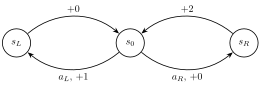
From , action leads deterministically to with reward , and action leads deterministically to with reward . From (resp. ), any action returns to with reward (resp. ).
Let denote the policy that always selects , and the policy that always selects .
Exercise 2.1. Using the Bellman equation from Exercise 1.1, verify that
Solution
Under all transitions are deterministic, so the Bellman equation collapses to
Substituting the second into the first gives , hence
Similarly, under :
Substituting yields , hence
Exercise 2.2. Determine the best action from state as a function of the discount factor . Show that the breakeven point is .
Solution
Since any action from or deterministically returns to with the same reward, the value of any policy at is determined entirely by the action chosen at . Hence comparing and suffices:
Since for , the sign is determined by :
- : is optimal — the immediate reward of outweighs a discounted future reward of .
- : is optimal — the agent is patient enough to wait one step for the larger reward.
- : both actions are equally good (breakeven), and each gives .
3. Bellman operators and the existence of optimal policies
Banach fixed-point theorem
In this and the following exercises, we will make use of the well-known Banach fixed point theorem:
Theorem 3.1 (Banach Fixed Point Theorem). Let be a complete metric space and let be a contraction mapping, i.e. there exists such that
Then has a unique fixed point satisfying . Moreover, for any initial point , one
has where is the -fold composition of with itself. That is, converges to with respect to the metric .
The problem
Definition 3.2 (Bellman optimality operator). Let denote the vector space of value functions, equipped with the sup-norm . The Bellman optimality operator is defined by
Exercise 3.1. Let be real-valued functions on a finite set . Prove that
Solution
Without loss of generality, assume . Let . Then:
Exercise 3.2. Using Exercise 3.1, prove that is a contraction mapping with contraction factor , i.e. for all ,
Solution
Fix an arbitrary state . Define for each :
Then and . By Exercise 3.1:
where the last step uses . Since this holds for every , taking the maximum over gives .
Exercise 3.3. Using Theorem 3.1, conclude that there exists a unique satisfying , and that for any initial , the iterates as .
Solution
The space is a finite-dimensional normed vector space, hence complete. By Exercise 3.2, is a contraction on with factor . Theorem 3.1 then gives the existence of a unique fixed point , and convergence for any .
Exercise 3.4. Show that for any policy , the operator defined by
Bellman Policy Operator
is also a contraction with factor . Conclude that is its unique fixed point and that for any initial as .
Remark. This shows that the numerical policy evaluation algorithm from the ARENA materials converges to the correct solution.
Solution
Fix and an arbitrary state . Then:
where the last step uses and . Taking the maximum over gives , so is a contraction with factor .
By Theorem 3.1, has a unique fixed point. By the Bellman equation (Section 1), satisfies , so is this unique fixed point. The convergence statement also follows from Theorem 3.1.
Exercise 3.5. Let be any value function, and let be a greedy policy with respect to , i.e.
Show that .
Solution
Since is deterministic, , so the sum over in collapses to the single term . For every :
where the second equality holds because selects a maximizing action by definition.
Exercise 3.6. Define the greedy policy with respect to by as in the previous part. Show that , i.e. the value function of equals the fixed point of .
Hint: show that satisfies the same fixed-point equation as .
Solution
We have by Exercise 3.5 and Exercise 3.3. So is a fixed point of . By Exercise 3.4, is the unique fixed point of . Therefore .
Exercise 3.7. Conclude that is an optimal policy: for every policy and every state ,
Hint: show that pointwise, then iterate and take the limit.
Solution
Let be any policy. Since the max over actions is at least as large as any weighted average:
In particular, since is a fixed point of (Exercise 3.4):
Note that is monotone: if for all , then . Applying to both sides and using monotonicity, then iterating:
By Exercise 3.3, as . Taking the limit:
where the last equality is Exercise 3.6. Since was arbitrary, is optimal.
4. Policy improvement theorem
Given a policy , define the improved policy greedily with respect to :
Policy Improvement
Exercise 4.1. In proving Exercise 3.7, we already saw that for all , we have . When does equality hold for all states?
Solution
We have
where we used the Bellman equation in the last step. If equality holds at every state , then is a fixed point of , which by uniqueness (Exercise 3.3) means , i.e. is already optimal by Exercise 3.7.
Exercise 4.2. Show that for all .
Hint: show that pointwise using Exercise 3.5, then iterate and take the limit.
Solution
By Exercise 3.5, pointwise, where the inequality is from Exercise 4.1. Note that is monotone: if for all , then . Applying to both sides and iterating:
By Exercise 3.4, as . Taking the limit gives for all .
Exercise 4.3. The policy iteration algorithm generates a sequence of policies where each is the greedy policy with respect to . Show that this sequence converges to an optimal policy in a finite number of steps.
Hint: how many deterministic policies are there?
Solution
By Exercise 4.2, the sequence of value functions is monotonically improving: for all and all . Since each is a deterministic policy and there are only deterministic policies, the sequence must eventually revisit a policy. If for some , then , and by monotonicity . In particular .
It remains to show this implies optimality. Since is greedy with respect to , Exercise 3.5 gives . Since is the fixed point of and , we get . Combining: , so is optimal by Exercise 4.1.
5. Bellman convergence rate
Exercise 3.3 showed that the iterates converge to for any starting , but it did not tell us how fast, nor how to decide when to stop iterating. We derive some convergence rate bounds (Puterman 1994, Chapter 6).
Exercise 5.1. Show that for any initial , the iterates satisfy
Remark. This bound is not useful as a stopping criterion in practice as it depends on the unknown .
Solution
Exercise 5.2. Show the a priori bound:
This bound uses only — a quantity computable after a single iteration, independent of .
Hint: write (valid since ), and bound each term using the contraction of .
Solution
By the contraction property applied repeatedly,
Since (Exercise 3.3), we have the telescoping identity . Applying the triangle inequality and the geometric bound above:
Exercise 5.3. Show the a posteriori bound: for ,
Hint: telescope from as in Exercise 5.2, but bound in terms of instead.
Solution
Step 1: bound each successive difference in terms of . Apply the contraction property of once:
Apply it again, chaining with the previous bound:
Continuing this pattern, for every :
Step 2: telescope. Since (Exercise 3.3), we have the telescoping identity
Applying the triangle inequality and the bounds from Step 1:
Exercise 5.4. Show that the a posteriori bound of Exercise 5.3 is always at least as tight as the a priori bound of Exercise 5.2: for all ,
Hint: bound by repeated application of the contraction.
Solution
Apply the contraction property of to and :
Continuing this times altogether, we eventually land on :
Multiplying both sides by preserves the inequality:
Both bounds from Exercise 5.3 and Exercise 5.2 upper-bound , and the a posteriori one is smaller.
Exercise 5.5. Assume for all . Show that if we initialize with , then
This bound depends only on , , and , so it can be evaluated before running a single iteration.
Solution
With :
Each term is a convex combination of rewards, all bounded in absolute value by , so for every , hence . Substituting into the a priori bound of Exercise 5.2:
Exercise 5.6. Show that the bound of Exercise 5.5 is tight: exhibit an MDP in which for every (with ).
Solution
Take , , , and . The Bellman optimality operator collapses to
Starting from and iterating,
The fixed point solves , giving . Therefore
so the bound of Exercise 5.5 is attained with equality. No bound in terms of only , , and can be sharper.
Remark. Combining Exercise 5.3, 5.2 and 5.5 gives a chain of progressively weaker but increasingly upfront-computable bounds:
Convergence Bounds
Each step weakens the bound by replacing realized information with something coarser: first the most recent step size with the worst-case geometric decay (contraction of applied times), then the initial step size with the crude reward bound . In practice the leftmost bound is significantly tighter, since often decays strictly faster than . It also yields a concrete stopping rule: to guarantee , iterate until .
6. Convergence of Q-learning
The policy improvement theorem from Section 4 shows that we can in principle find an optimal policy in MDPs. However, it makes the uncomfortable assumption that we know the environment dynamics via the transition kernel . In this problem, we prove that -learning, which does not make such an assumption, converges to the optimal action-value function, from which one can trivially extract an optimal policy by choosing actions greedily.
Stochastic approximation theorem
We will make use of the following stochastic approximation result, which we state without proof:
Theorem 6.1 (Stochastic Approximation for Contractions (Tsitsiklis 1994, Theorem 3)). Let be the space of real-valued functions on a finite set , equipped with the sup-norm . Let be a contraction mapping with factor and unique fixed point .
Fix an initial iterate , and for each let be a learning rate function and a random noise function (both functions on , one value per coordinate). Consider the stochastic iteration
where updates are applied to a single coordinate at each step (i.e. for ). Suppose:
(a) (Learning rate) For each :
(b) (Noise) For each , conditioned on the history , the noise has zero mean and bounded variance:
for some constant .
Then for all , with probability .
What is stochastic? The randomness of the iteration is carried by the noise: each is a real-valued random variable, and is a random element of . Consequently, the iterates are random (they depend on past noise ), and the learning rates may be random as well if they depend on the history—e.g. on which coordinate was just visited. The contraction , its fixed point , the update rule itself, and the initial iterate are all deterministic. The theorem asserts that despite the noise, the random sequence converges pointwise to almost surely.
Remark on "with probability ". The conclusion with probability (also called almost sure convergence) means
In other words, the probability that a run of the stochastic iteration fails to converge to is zero.
Why should we believe this? It helps to build up the result in three layers of increasing complexity.
Layer 1: no noise, all coordinates at once. If and for all and , the iteration reduces to . This converges to by Theorem 3.1.
Layer 2: noise, but all coordinates at once. Now suppose we observe instead of , and use a decreasing step size:
The signal always points toward (this is what the contraction property buys us). The noise is mean-zero, so it pushes us in random directions that partially cancel over time. The two conditions on the step size mediate between signal and noise:
- ensures the total step size is large enough to reach from any starting point.
- ensures the noise averages out. Each noise term enters the iteration scaled by , contributing a random displacement of size . Although these displacements are not independent (each depends on the current iterate ), they are mean-zero conditioned on the past. For such sequences, the variance of the cumulative sum is the sum of the individual variances, which is proportional to . Since this is finite, the total random drift converges and cannot overwhelm the steady pull of the signal toward .
The signal accumulates coherently (always pulling toward ), while the noise averages out.
Layer 3: one coordinate at a time. The iteration updates only one coordinate per step, while the others stay frozen. This makes the analysis more difficult since the target depends on all coordinates, including stale ones. The condition for each ensures no coordinate is permanently neglected, and the contraction property of provides enough global coupling to prevent coordinates from drifting apart. Making this rigorous is the main technical content of the proof.
The problem
Consider the following generalization of the Q-learning update from the ARENA materials, now with a time-varying learning rate : given a current estimate and an observed transition where and , the update is
Q-Learning Update
with for all . We will show that, under appropriate conditions, Q-learning converges to the optimal action-value function .
Let denote the space of action-value functions, equipped with the sup-norm .
Exercise 6.1. Overloading the notation from Definition 3.2, define the Bellman optimality operator on action-value functions, , by
Bellman Q-Operator
(Here takes a -function to a -function, whereas the earlier in Definition 3.2 takes a -function to a -function — whether denotes the - or -version is always clear from its argument.) Show that is a -contraction on .
Hint: this is similar to the proof of Exercise 3.2.
Solution
Fix and . By the inequality from Exercise 3.1 (applied at each ) and the triangle inequality:
Taking the maximum over gives .
Exercise 6.2. Define , the action-value function of the optimal policy from Section 3. We now show Bellman optimality equations and their consequences.
(a) Show that .
(b) Show that .
(c) Conclude that is the unique fixed point of .
Solution
(a) By Exercise 1.2(b) applied to :
By Exercise 3.6, . Substituting gives the result.
(b) By Exercise 1.2(a), . Since is the greedy policy with respect to (Exercise 3.5 and 3.6), it is deterministic and selects . By Exercise 6.2(a), the inner expression equals , so . Since is deterministic, .
(c) Substituting Exercise 6.2(b) into Exercise 6.2(a):
So is a fixed point of . Uniqueness follows from Exercise 6.1 and Theorem 3.1.
Exercise 6.3. Rewrite the Q-learning update in the form of Theorem 6.1:
Specifically, identify the index set , the mapping , the iterates , and the learning rates . Then give an explicit expression for the noise .
Solution
The identifications are:
- Index set: .
- Iterates: .
- Contraction: , with fixed point (Exercise 6.2).
- Learning rates: .
With these identifications, the Q-learning update becomes
where the noise at the updated coordinate is
i.e. the difference between the sampled target (using the single transition ) and its expectation over all possible transitions. For , we set .
Exercise 6.4. Show that the noise satisfies for all , where denotes the history up to time as in Theorem 6.1.
Hint: conditioned on , the quantities , , and are all determined. What is the only remaining source of randomness?
Solution
Conditioned on , the quantities , , are all determined. The only remaining randomness is in . Therefore:
For , we have by definition, so trivially.
Exercise 6.5. Assume for all . Show that there exists a constant (depending only on and ) such that
Hint: first show that .
Solution
Step 1: a pointwise bound on . Using and , the sampled target satisfies
The same bound holds for , since it is a convex combination (over ) of terms each bounded by . By the triangle inequality:
This bound holds for every realization of , not just in expectation.
Step 2: passing to the conditional second moment. Squaring the pointwise bound,
Taking conditional expectation of both sides given preserves the inequality (monotonicity of conditional expectation):
Now we simplify the right-hand side. It is a function of (and the constants ), and is determined once we condition on (recall records ). So the right-hand side is -measurable: given the history, it is a fixed real number, not random. Conditional expectation acts as the identity on -measurable quantities — i.e. when is -measurable — so
Combining,
Step 3: putting it in the required form. We want a constant such that the right-hand side is bounded by . Applying with , :
So works. For , we have , so the bound holds trivially with the same .
Exercise 6.6. Conclude: state the conditions on the learning rate schedule and the exploration policy under which Q-learning converges, i.e. with probability . Remark. The ARENA implementation uses a constant learning rate , which does not satisfy . In practice, constant-rate Q-learning does not converge exactly but oscillates in a neighbourhood of whose size shrinks with .
Solution
By Exercises 6.1–6.5, the Q-learning iteration satisfies all the hypotheses of Theorem 6.1, provided the learning rate conditions hold: for each ,
Under these conditions, Theorem 6.1 gives with probability .
Note that the first condition already implies that each state-action pair must be visited infinitely often. A concrete way to achieve all three conditions is to use an exploration policy that visits every infinitely often together with a per-coordinate learning rate , where counts the number of visits to up to time . This satisfies and .
7. Exact policy evaluation
In Exercise 3.4, we showed that iterating converges to ; this is the numerical policy evaluation scheme used in the ARENA materials. When the state space is finite and the dynamics are known, there is also an exact (closed-form) solution: the Bellman equation becomes a linear system that can be solved directly. In this problem we derive that closed form for deterministic policies.
Definition 7.1 (Matrix-vector notation for a deterministic policy). Fix a deterministic policy . Treating the value function as a vector in , define:
- with ,
- with (the transition matrix under ),
- with (the reward matrix),
- with (the expected immediate reward).
Fact 7.2 (Neumann series). Equip with the induced -norm
If , then is invertible, and
Exercise 7.1. Starting from the Bellman equation (Exercise 1.1) applied to a deterministic policy , show that
Exact Policy Evaluation
assuming is invertible (which we prove in Exercise 7.2).
Hint: specialize the Bellman equation to a deterministic policy and write the resulting system of equations in matrix-vector form.
Solution
Since is deterministic, , and the Bellman equation from Exercise 1.1 collapses the sum over actions:
Splitting the reward and value terms and rewriting with the matrix notation of Definition 7.1:
This holds for every , so in vector form
Assuming is invertible, left-multiplying by its inverse gives .
Exercise 7.2. Prove that is invertible for any deterministic policy and any .
Hint: apply Fact 7.2.
Solution
The matrix is row-stochastic: and for every . Therefore
and so . By the Neumann series (Fact 7.2), is invertible, with
Combining with Exercise 7.1,
which has a direct interpretation: is the vector of expected rewards exactly steps into the future under , and is their discounted sum.
Remark. The same derivation extends to stochastic policies by defining and . The matrix remains row-stochastic, so the argument above applies unchanged.
References
M. L. Puterman (1994). Markov Decision Processes --- Discrete Stochastic Dynamic Programming. Wiley.
John N. Tsitsiklis (1994). Asynchronous Stochastic Approximation and Q-Learning. Machine Learning.
Footnotes
-
Noting that is a finite set, this implies that the rewards are bounded above by . ↩